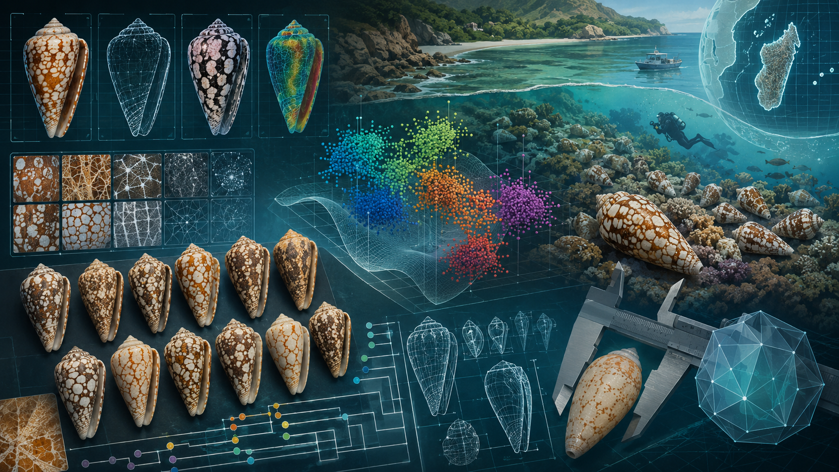
Phenotypic Structure in the Conus pennaceus Complex: Integrating Interpretable Morphometrics and Self-Supervised Image Embeddings
Published on: August 2026

Abstract
Shell morphology remains central to the taxonomy of Conus, but conspicuous phenotypic variation does not necessarily correspond to species boundaries. We investigated morphological structure in the Conus pennaceus complex using a frozen photographic dataset of 1,000 physical specimens, combining 41 interpretable shell traits with label-independent DINOv3 embeddings of RGB phenotype, binary silhouette and luminance-normalized surface pattern. Repeated photographs were resolved to physical specimens or specimen–view units, and anatomical view, repository provider and geography were evaluated before taxonomic comparisons. Currently accepted species were first compared with an operational C. pennaceus sensu-stricto reference to establish empirical morphological benchmarks; synonymized and unresolved forms were then evaluated within the same framework.
Embedding principal components showed strong correspondence with recognizable shell characters, but generally represented composite phenotype axes rather than individual traits. RGB and normalized-pattern embeddings described an almost identical surface-phenotype structure, whereas outline shape was substantially more independent. Observational structure was important: anatomical view accounted for much of a conspicuous two-band morphometric pattern, and provider effects exceeded broad geographic effects. Within the current Madagascar–Mozambique sensu-stricto analysis, geography explained 1.86% of multivariate trait variance after provider adjustment, compared with 23.40% for provider source.
Morphological recovery varied markedly among accepted species. C. vezoi showed strong multidimensional differentiation, C. bazarutensis and C. rubropennatus showed repeatable but overlapping phenotypes, and C. praelatus, C. quasimagnificus and C. episcopus showed more limited differentiation; C. ganensis and C. lohri were underpowered. In contrast, the currently synonymized C. elisae (N = 95) showed strong differentiation in all embedding representations and 28 FDR-supported measured traits, placing its shell phenotype within the strongest range observed among accepted-species benchmarks. Individual specimens nevertheless showed substantial shape–surface discordance and morphological mosaicism.
Within 595 operational sensu-stricto specimens, a joint shape–pattern Gaussian-mixture analysis reproducibly preferred two candidate components, but the same procedure selected multiple components in every heavy-tailed continuous-null simulation. Under the prespecified decision rule, candidate K = 2 therefore remained supported K = 1, indicating structured internal heterogeneity without demonstrated recurrent discrete morphotypes.
These results show that interpretable morphometrics and self-supervised image embeddings provide complementary evidence for complex shell phenotype, while also demonstrating that morphological differentiation, taxonomic rank and species status are distinct quantities. The recovered phenotypes provide testable hypotheses for subsequent type-based, molecular, anatomical, ecological and geographically replicated validation rather than morphology-only species delimitations.
Introduction
Shell morphology has played a central role in the taxonomy of Conus, but the relationship between conspicuous shell variation and species boundaries is not straightforward. This problem is particularly evident in the Conus pennaceus Born, 1778 complex, in which variation in shell proportions, spire and shoulder geometry, pigmentation and reticulated surface pattern has historically been described through a mixture of species, subspecies, synonyms and named forms. Treatments of these names have changed through time, and the taxa represented in the present complex consequently include currently accepted species as well as names treated as synonyms or retained only as historical or project-level phenotype labels [1, 5]. Morphological differentiation and nomenclatural status must therefore be distinguished: a reproducible shell phenotype can be taxonomically informative without, by itself, demonstrating an independently evolving species lineage [15, 16].
Geographic variation adds a further dimension to this problem. Historical work on the C. pennaceus complex has emphasized geographically differentiated shell forms in the western Indian Ocean, including Madagascar and the Mozambique region [5]. The most directly relevant molecular study of Mozambican material was performed by Pereira et al., who analysed mitochondrial 12S and 16S rRNA sequences from 22 specimens sampled along the Mozambican coast and recovered geographic structure within the complex [23]. That study provided important evidence that geography and evolutionary history are relevant to the observed shell diversity, but its small sample and reliance on two mitochondrial loci did not constitute an integrative or genome-scale delimitation of the shell phenotypes represented in the complex. Subsequent molecular and phylogenomic studies have greatly strengthened the evolutionary framework for Conidae as a whole [24, 25, 26], but they have not provided geographically dense population-level evidence resolving the correspondence between the principal pennaceus-complex shell phenotypes and independently evolving lineages.
Quantitative shell morphology therefore remains an important evidence layer. Kohn and Riggs established a geometric framework specifically for the Conus shell, showing that shell length, relative diameter, spire geometry and the position of maximum diameter can be represented quantitatively rather than through qualitative descriptors alone [2]. Geometric morphometrics subsequently extended this approach to the spatial organization of shell shape. In Conus, Cruz, Pante and Rohlf demonstrated that landmark-based morphometric spaces can discriminate species and that variation involving the spire, shoulder and aperture contributes substantially to interspecific shell-shape differences [3]. Morphometric analysis has also been used more recently in the taxonomic reassessment of other Conus species, illustrating the continuing value of quantitative shell form as evidence in systematic problems [27].
Conventional morphometrics, however, describes only selected aspects of a phenotype that is visually much richer. The C. pennaceus complex combines variation in overall shell geometry with spatially complex pigmentation, reticulation, local pattern density and colour. High-dimensional image representations provide a complementary means of describing such variation without requiring every potentially informative feature to be specified in advance. Self-supervised vision models are particularly attractive for this purpose because a pretrained encoder can generate image representations without being trained on the taxonomic or phenotype labels subsequently examined. DINOv3 provides such frozen transferable visual representations [4]. The literature searches undertaken for the present study did not identify a peer-reviewed application of DINOv3 specifically to morphological species delimitation in Conus, making its use here an extension of established quantitative shell morphometrics rather than a replacement for it.
High-dimensional embeddings nevertheless require biological validation and careful control of observational structure. A visual representation can encode shell shape and pigmentation while simultaneously retaining differences associated with anatomical projection, image source, photographic conditions or geographic sampling. Likewise, apparent separation of predefined labels in an embedding space does not establish species boundaries, particularly when those labels have complex historical provenance or have been subject to subsequent review. For this reason, interpretable shell measurements and image embeddings are most informative when their biological correspondence is quantified explicitly, when repeated photographs are reduced to the physical specimen as the independent biological unit, and when anatomical view, provider and geography are evaluated before taxonomic separation is interpreted. Morphological evidence can then contribute to an integrative taxonomic hypothesis while remaining conceptually distinct from genetic, reproductive, ecological or nomenclatural evidence [15, 16].
The present study applies this framework to a frozen photographic dataset of 1,000 physical specimens associated with the C. pennaceus complex. Shell phenotype is described in two complementary ways: directly interpretable physical and image-derived traits, and high-dimensional DINOv3 representations of the complete RGB phenotype, shell silhouette and luminance-normalized surface pattern. Rather than asking whether an image classifier reproduces existing names, the study asks how shell phenotype is structured, which biological traits are represented by the embedding spaces, and how much of the observed variation is associated with anatomical view, repository provider and geography before taxonomic labels are considered.
The principal taxonomic question is then approached comparatively. Currently accepted species represented by sufficient numbers of independent specimens are first evaluated against an operational C. pennaceus sensu-stricto reference to establish empirical benchmarks for shell differentiation. Historical synonyms and unresolved forms are subsequently evaluated using the same framework rather than being assumed a priori either to be distinct or to be morphologically equivalent to C. pennaceus. The analysis further examines whether differentiation is integrated across shell shape and surface phenotype, whether individual shells show discordant or mosaic combinations of these components, and whether the operational sensu-stricto population itself contains evidence for recurrent discrete morphological components rather than continuous internal variation.
The aim is therefore not to derive formal species boundaries from shell photographs alone. It is to establish, on a common quantitative basis, which named and unnamed components of the C. pennaceus complex correspond to repeatable shell phenotypes, how those phenotypes are expressed across interpretable morphology and image-derived feature spaces, and how strongly their apparent differentiation persists after major observational sources of variation are taken into account. This provides a morphology-based evidence framework that can subsequently be tested against type material, geographically replicated sampling and independent molecular, anatomical and ecological evidence.
Materials and methods
Study design and analytical sequence
Study objective and inferential scope
The study was designed as a morphology-based assessment of phenotypic variation within the Conus pennaceus complex. Its purpose was not to infer species status directly from current taxonomic names, image classifications or visual clusters, but to determine whether currently accepted species, historical synonyms and project-level forms were associated with repeatable differences in shell phenotype. Morphological evidence was quantified from both directly interpretable shell traits and high-dimensional image embeddings representing combined RGB phenotype, silhouette shape and luminance-normalized surface pattern.
Three levels of information were therefore kept conceptually separate throughout the study: nomenclatural status, representing the current treatment of a name in MolluscaBase/WoRMS; phenotype labels, representing identifications inherited from source records or subsequently assigned during project review; and morphological evidence, representing the measurements and statistical results generated from the shell images. Current nomenclatural status was used to organize the analytical sequence, but was not treated as a morphological ground truth. This distinction is consistent with the broader principle that morphological diagnosability and taxonomic naming are evidence relevant to species delimitation but are not, by themselves, demonstrations of independently evolving lineages [1, 15, 16].
Phenotype labels and taxonomic status
Two phenotype-label fields were retained for each physical specimen. The
original_variant field preserved the name reconstructed from the source record,
whereas assigned_variant recorded a later project identification where one had
been made. The effective phenotype label used in the frozen analytical dataset was the assigned
variant when present and otherwise the original variant. Specimens for which neither field
contained a named form were assigned to the operational
C. pennaceus sensu-stricto reference group.
Assigned variants were determined by visual review of the shell images and, in some cases, information from the project analyses was also available during that review. Original source-derived labels were retained rather than overwritten. Consequently, assigned phenotype labels were treated as curated phenotype hypotheses and audit information, not as an independent reference standard against which the same image-derived morphology could be validated. The operational sensu-stricto group likewise denotes the residual unqualified pennaceus phenotype group in the frozen dataset and does not imply comparison of every specimen with type material or material from the type locality.
Current taxonomic interpretation was reconciled separately against MolluscaBase/WoRMS using the taxonomic snapshot defined for the study [1]. Names corresponding to accepted species, names currently treated as synonyms, and unresolved project-level forms were therefore retained as distinct analytical categories even when their present nomenclatural status differed. This allowed the morphological behaviour of historically recognized phenotypes to be evaluated without converting current database acceptance or synonymy into a prior assumption about their expected morphological separation.
Accepted-species-first analytical design
Taxonomic group comparisons followed an accepted-species-first design. Operational C. pennaceus sensu stricto served as the common morphological reference. The first taxonomic stage compared sufficiently represented labels corresponding to currently accepted species with this reference. These comparisons established empirical benchmarks for the amount and type of shell differentiation recovered from taxa already recognized at species rank. Recovery of a distinctive shell phenotype was interpreted as morphological support for the recorded identification; absence of strong shell separation was not interpreted as evidence against the accepted taxonomic status of a species.
Only after these benchmarks had been established were names currently treated as synonyms and unresolved or informal project forms evaluated. Their shape, surface phenotype and directly measured trait differences were assessed using the same analytical framework and compared descriptively with the range of differentiation observed among the accepted-species benchmarks. The analysis did not perform an aggregate statistical test of “accepted species” against “synonyms” as taxonomic classes, and no universal morphological separation threshold was assumed to define species.
Sequential analysis of phenotype evidence
The statistical analyses followed the same hierarchy. First, the overall structure of measured shell phenotype was characterized without interpreting named groups. Trait distributions, correlations and redundancy were examined, a primary multivariate trait space was constructed, and associations between directly measured biological traits and embedding principal components were quantified. This established what biological information was represented by the image-derived feature spaces before those representations were used for taxonomic comparisons.
Second, anatomical view, repository provider and geography were examined as potential non-taxonomic contributors to phenotype structure. These analyses preceded interpretation of named groups because dorsal and apertural projection, photographic source and regional sampling could otherwise produce apparent separation unrelated to taxonomic identity. Provider-adjusted and view-aware analyses were therefore used where specified by the individual statistical procedures.
Third, sufficiently represented currently accepted species were compared separately with the operational sensu-stricto reference. Fourth, synonymized and unresolved form labels were evaluated using the same embedding and directly measured trait evidence. This ordering provided an empirical reference for interpreting the magnitude and multidimensional character of differences recovered among historical forms without assuming that their current nomenclatural rank predicted the result.
Fifth, analyses moved from the magnitude of group separation to the architecture of that separation. Correspondence among the RGB, shape and pattern representations was quantified independently of taxon labels, after which group labels were overlaid to determine whether differentiation was expressed across several phenotype modules or was concentrated in a particular component such as shell outline or surface pattern. Individual specimens were then examined for cross-stream discordance and nearest-group resemblance. Original and assigned labels, provider, anatomical view and locality were retained as descriptive audit information during this specimen-level inspection.
Finally, internal structure was examined within the operational C. pennaceus sensu-stricto group itself. This analysis was restricted to specimens already frozen as sensu stricto before unsupervised mixture discovery. Candidate structure was evaluated independently in shape, surface and joint phenotype spaces, and named forms were considered only afterward for interpretation of any candidate components. The complete sequence ended with an integrated morphological summary combining sampling adequacy, multivariate embedding separation, directly measured trait differences, phenotype-module architecture, individual overlap and internal consistency. The resulting assessments describe shell-phenotype evidence and were not used to make formal nomenclatural acts.
Design principle. The analysis therefore proceeded from comparatively assumption-light description of phenotype structure toward progressively more taxonomically explicit questions. Current taxonomic rank determined the order in which hypotheses were evaluated, but morphology was analysed as evidence rather than being required to reproduce the nomenclatural classification.
Dataset construction and taxonomic composition
Assembly of the photographic dataset
A photographic dataset was assembled for specimens identified as Conus pennaceus Born, 1778 or as named forms and species historically associated with the C. pennaceus complex. Records originated from 32 provider categories representing a heterogeneous mixture of online catalogues, auction records, biodiversity repositories, field guides and project collections. Consequently, the dataset constitutes an observational convenience sample rather than a spatially randomized or population-stratified survey.
Each database record represented a putative physical shell specimen. Available photographs were linked to this specimen record and then passed through the image eligibility, segmentation, view-classification and standardization pipeline described below.
Image eligibility and construction of visual representations
Photographs entered the image-processing pipeline only when they were recorded as original images, had an available local image file and had not previously been rejected during source-image quality control. No adult/juvenile or shell-condition eligibility criterion was applied. Eligibility at this stage was therefore determined by image availability, subsequent shell detection and segmentation, anatomical view and the quality-control decisions described below.
Shell detection, segmentation and crop review
Shell instances were detected and segmented using the project YOLO segmentation model. For every detected instance having a non-empty segmentation mask, the mask was rasterized at the dimensions of the source photograph and used to isolate the detected shell from its background. A crop was constructed from the bounding extent of the mask with additional surrounding padding, and pixels outside the mask were set to black. The resulting crop was placed on a square black canvas. Processing provenance, detection confidence, bounding-box geometry, mask area and crop geometry were retained for quality control.
Images containing more than one detected shell were not resolved by automatically choosing a single detection. Instead, every detection with a valid non-empty mask generated a separate candidate shell crop, and the presence of multiple detections was recorded as a warning attribute. The preprocessing stage likewise recorded diagnostic flags for potentially problematic detections, including low-confidence detections, comparatively small detected shells and implausible relationships between mask and bounding-box area. These flags were used to support review rather than as automatic biological exclusion criteria. Images for which no shell was detected, or detections for which no usable mask crop could be generated, did not produce a candidate shell image for subsequent processing.
Candidate masked crops were inspected manually. The review interface allowed each transformed shell image to be accepted, rejected or returned to an unreviewed state, with an optional explanatory note. Final image-quality decisions were based on reviewer judgement rather than on an additional fixed numerical acceptance rule. A rejected crop was marked as unavailable for analysis and was excluded from subsequent processing. Automated diagnostic flags therefore identified images requiring attention but did not replace manual quality assessment.
Classification of anatomical view
Anatomical view was assigned manually to each non-rejected detected shell. An apertural view was operationally defined as a view in which the aperture and outer lip were clearly visible. A dorsal view represented the side opposite the aperture, equivalent to the abapertural surface. The review system additionally allowed left-lateral, right-lateral, apical, basal, oblique-apertural, oblique-dorsal, uncertain and other views to be recorded rather than forcing every photograph into one of the two analytical views.
Each view assignment also carried a confidence category. Only dorsal or apertural detections classified with certain or probable confidence were eligible for orientation and subsequent phenotype analysis. Unknown or uncertain classifications, lateral views, apical and basal views, oblique views and other unsupported projections were excluded from the analytical image pipeline. This restriction was imposed because shell projection affects apparent outline, shoulder geometry and the position of measurable structures. Dorsal and apertural views were subsequently retained as distinct observations rather than treated as interchangeable photographs [2, 3].
Long-axis orientation and apex standardization
Eligible dorsal and apertural masks were standardized automatically to an apex-up orientation. The principal long axis of the segmented shell was estimated from the spatial distribution of mask pixels using principal-component geometry. Widths perpendicular to this axis were then evaluated along the shell, and the position of the widest supported perpendicular chord was used to resolve the otherwise arbitrary direction of the principal axis. The end of the long axis lying closer to this maximum-width position was provisionally identified as the apex. The image and its mask were then rotated so that the inferred apex pointed upward.
Orientation diagnostics quantified the stability of the long axis, maximum-width chord and apex assignment. Ambiguous geometry or low overall confidence generated review flags rather than an automatic taxonomic decision. Every oriented image could subsequently be inspected together with a diagnostic preview showing the calculated long axis, maximum-width chord and inferred apex.
Rotation was performed without horizontal reflection. Before rotation, the masked shell was surrounded by additional black safety padding so that a shell reaching the edge of its original photograph was not clipped by the rotation operation. After rotation, the smallest bounding rectangle containing the shell was extracted and centred on a square black canvas sized to retain a minimum margin around the shell. The resulting image therefore standardized the apex-to-base axis and shell position while preserving the original chirality of the photograph.
Oriented outputs were reviewed manually and could be accepted, rejected or corrected. When correction was required, the review workflow allowed an additional angular adjustment and/or a 180° reversal of the inferred apex direction. A correction generated a new versioned derivative while preserving the earlier result; images were not overwritten. Only accepted, analysis-ready orientation results were eligible for construction of the final visual representations.
Construction of colour, shape and pattern representations
Each accepted orientation served as the common geometric reference for three aligned image representations. The RGB representation was the accepted oriented colour image itself and therefore retained the combined visible phenotype, including shell outline, pigmentation, pattern and any remaining variation in image acquisition. The shape representation was a binary silhouette reconstructed by applying the stored orientation transformation to the original segmentation mask. This ensured that the silhouette and RGB image occupied the same coordinate system and that the shape stream contained shell-mask geometry rather than colour or surface-pattern information.
The pattern representation was constructed from the accepted oriented RGB image within the same reconstructed shell mask. RGB values were converted to CIELAB colour space, and the luminance channel was normalized within the shell while the image remained spatially aligned with the RGB and shape representations. Pixels outside the shell mask were set to black. The transformation was intentionally partial rather than a replacement of the observed luminance distribution: its purpose was to reduce differences in overall illumination and brightness while retaining spatial pigmentation structure. The implementation used OpenCV for colour-space conversion [6] and the CIE 1976 L*a*b* representation described by McLaren [11]. Exact percentile, target-luminance and normalization-strength parameters are reported in the Supplementary Methods rather than treated as biological variables.
Representation generation included automated validation of the reconstructed mask and luminance transformation. Diagnostic warnings were recorded when, for example, the reconstructed mask contained multiple connected components, touched the canvas boundary, occupied an unusually small or large proportion of the canvas, or when the luminance normalization produced unusually large changes or clipping. As in the earlier processing stages, these diagnostics prompted inspection but did not substitute for the final review decision.
Independent representation quality control
The three visual streams were not accepted automatically as a package. The RGB image had already undergone orientation review, while the generated shape and pattern derivatives were presented separately for quality assessment and could each be accepted or rejected independently. Review decisions were propagated to the corresponding transformed-image records, and rejected derivatives were marked as unavailable for analysis.
An image lineage became eligible for embedding extraction only when the oriented RGB image was accepted and analysis-ready and both the aligned shape and pattern derivatives were also accepted and analysis-ready. Missing, rejected, failed or still-unreviewed members therefore prevented that lineage from entering the three-stream analytical cohort. This requirement ensured that subsequent RGB, shape and pattern comparisons were based on matched representations of the same accepted shell image rather than on partially overlapping image sets.
Definition of the analytical unit
The frozen dataset contained 2,385 accepted colour–shape–pattern representation triplets. Repeated photographs of the same physical specimen in the same anatomical view were not treated as independent observations. Their embedding vectors were averaged within specimen and view, and the resulting mean vector was normalized again. This reduced the dataset to 1,862 specimen-view units derived from 1,000 physical specimens. Of these units, 934 were apertural and 928 were dorsal. Both views were available for 862 specimens; 72 specimens had only an apertural view and 66 only a dorsal view.
When a database duplicate group identified records as photographs of the same physical shell, the duplicate group—not the individual database row—defined the specimen. Otherwise, the specimen identifier was used. This duplicate-aware construction prevented repeated photographs from inflating sample size while preserving complementary dorsal and apertural information.
Embedding extraction and dimensionality reduction
Frozen DINOv3 feature extraction
Image embeddings were extracted separately for the RGB, shape and pattern
representations using the pretrained DINOv3 ViT-S/16 preset
dinov3_vit_small_lvd1689m
[4]. The backbone was loaded through TensorFlow/KerasHub
and kept frozen throughout feature extraction
(trainable = False). Each model input had dimensions
336 × 336 pixels and three channels.
RGB and pattern images were converted to RGB and resized to 336 × 336 pixels using bilinear interpolation. Binary shape images were converted to a single grayscale channel, resized using nearest-neighbour interpolation and then repeated across three channels. The registered DINOv3 image converter supplied with the preset was subsequently applied before inference. No additional augmentation was applied during embedding extraction.
The DINOv3 backbone returned a sequence of token representations for each image. The first token, corresponding to the class token (CLS token), was retained as the global image representation. This produced one 384-dimensional float32 embedding for each accepted image and representation stream. Both the unmodified 384-dimensional vector and a separately L2-normalized version were stored. The normalized vectors were used when repeated photographs were aggregated into the specimen–view units defined above.
Independence from project phenotype assignments
The encoder was not trained, fine-tuned or otherwise fitted to the phenotype assignments in this project. Pretrained DINOv3 weights were loaded from the registered preset and remained unchanged during extraction. Model input consisted only of the corresponding image representation; original or assigned variant labels, current taxonomic status, provider, anatomical view and geographic metadata were not supplied to the encoder. Project phenotype labels therefore played no direct role in construction of the embedding vectors.
Feature standardization and principal component analysis
Dimensionality reduction was performed after repeated photographs had been combined into the duplicate-aware specimen–view units described above. For each representation stream, the resulting analysis matrix therefore contained one row per specimen–view unit and 384 embedding dimensions. Before decomposition, the stored L2-normalized vectors were checked for the expected dimensionality, finite values and unit vector norm.
The 384 embedding dimensions were then standardized independently within each representation stream by subtracting the feature-wise cohort mean and dividing by the feature-wise standard deviation:
Principal component analysis (PCA) was fitted separately to the standardized RGB, shape and pattern matrices using full singular-value decomposition. Consequently, each visual representation had its own PCA basis, eigenvalues, explained-variance profile and specimen–view scores. Components from different streams were not assumed to be homologous; for example, RGB PC1 and shape PC1 denote the leading variance axis within their respective representations rather than the same biological dimension.
Component-retention rule
Cumulative explained variance was calculated across the complete PCA solution. The numbers of components required to reach 80%, 85% and 90% cumulative variance were recorded for diagnostic purposes. The primary inferential representation used the smallest number of components whose cumulative explained variance was at least 85%:
All PC scores from PC1 through the stream-specific k85 cutoff were retained. These retained multivariate coordinates, rather than only the first two or three principal components, formed the embedding representation supplied to subsequent statistical analyses. The 80% and 90% thresholds were recorded as dimensionality diagnostics but did not replace the prespecified 85% primary cutoff.
Exploratory nonlinear projections
Two-dimensional UMAP and t-SNE coordinates were also calculated independently for each representation stream from the standardized 384-dimensional embedding matrix. These projections were retained for exploratory visualization and image inspection only. They were not used to define the phenotype groups, select the number of PCA components, calculate multivariate effect sizes or perform hypothesis tests.
In particular, apparent clusters, gaps, overlap or relative spacing in a two-dimensional UMAP, t-SNE or PC1-versus-PC2 display were not treated as statistical evidence for morphological differentiation. Formal analyses used the retained PCA coordinates defined by the 85% cumulative-variance criterion. Exact projection parameters, run identifiers, software-version provenance and source-array checksum verification are reported in Supplementary Methods SM4.
Inferential rule. Dimensionality reduction was used to obtain a reproducible multivariate representation of each embedding stream, not to infer groups visually. Statistical conclusions were based on the retained PCA subspaces; nonlinear two-dimensional projections served only as exploratory displays.
Phenotype-label curation and analytical reference groups
Phenotype-label provenance was retained separately from later project review.
The field original_variant stored a form or taxon name reconstructed
from the source record, whereas assigned_variant stored a subsequent
reviewer assignment when one had been made. Curation therefore did not overwrite
the reconstructed source-derived label.
Reconstruction of source-derived phenotype labels
Original phenotype labels were reconstructed from the imported source data using a predefined vocabulary of historical and project-relevant names. Three source fields were examined in fixed order: the stored species name, the source webpage and the shell description. Text was URL-decoded and matched case-insensitively using name boundaries so that a variant name embedded within another word was not counted as a match.
The first source field containing exactly one recognized phenotype name supplied
the original_variant. The source field from which the name was
recovered and a truncated copy of the supporting source text were retained as
provenance. If a source field contained more than one candidate name, the record
was classified as conflicting and no original variant was inferred from that
record. Records for which no candidate name could be reconstructed remained
without an original_variant; absence of a recoverable label was not
converted into a named phenotype.
The reconstruction vocabulary comprised bazarutensis, colubrinus, confusa, convolutus, elisae, episcopus, ganensis, lohri, marmoricolor, mimeticus, praelatus, quasimagnificus, rubiginosus, rubropennatus and vezoi. This list defined names that could be recovered from source text; it did not imply that every name was represented in the final analytical cohort or currently accepted at species rank.
Preservation of earlier manual assignments
Before the two-field provenance scheme was introduced, manually assigned values
had been stored in a legacy variant field. During migration, an
existing legacy value was copied to assigned_variant only when an
assigned value was not already present. The migration did not alter the newly
reconstructed original_variant. Because the original review dates
of these legacy assignments were unavailable, migrated assignments were explicitly
annotated as having an unknown original assignment timestamp rather than being
given a reconstructed date.
Phenotype review and reassignment
Subsequent phenotype curation was based on reviewer judgement. All manual
phenotype-review and reassignment decisions were made by a single reviewer.
Specimens were inspected visually, and information from the project analyses
was available during some reviews. A reviewer could assign a new
assigned_variant, replace an existing assignment or clear the
reviewed assignment. Clearing assigned_variant did not alter
original_variant and therefore restored inheritance from the
source-derived label when one was available.
The general curation interface displayed the specimen images together with available specimen and provenance information, including the original variant, source of that original label, original identification, repository source, country and locality. Review time and a review note were stored for subsequent assignments. Thus, the source-derived and reviewer-derived components of the phenotype label remained distinguishable after curation.
A focused analysis-assisted review was additionally implemented for five sufficiently represented phenotype groups: C. pennaceus sensu stricto, vezoi, elisae, rubropennatus and bazarutensis. For this review, the interface could display cross-validated morphological resemblance scores calculated separately from the RGB, shape and pattern embedding streams and combined at physical-specimen level. The score-generation procedure kept all views of a physical specimen in the same cross-validation fold and produced out-of-fold scores. These quantities were explicitly defined by the implementation as balanced resemblance scores rather than prevalence-calibrated posterior probabilities.
The focused scores were review information rather than automatic assignment rules. The reviewer retained the final decision and could assign one of the five focused labels or clear the reviewed assignment so that the original label again became effective. Changes made through this focused workflow were recorded with the previous and new assignments, the assignment-analysis run, the model-suggested label and score, an optional reviewer note and the change time.
assigned_variant was treated as a curated phenotype hypothesis rather
than as an independent ground-truth label. Subsequent recovery of morphological
differences among these groups was therefore not interpreted as independent
validation of the review decisions.
Effective-label rule
Group-based analyses used a fixed precedence rule. A non-empty
assigned_variant superseded the reconstructed
original_variant. When no reviewed assignment was present, the
original variant was inherited. If neither field contained a named phenotype,
the specimen belonged operationally to the unqualified
C. pennaceus reference group.
assigned_variant
→
original_variant
→
C. pennaceus sensu stricto
At cohort-freezing time, the implemented effective-assignment contract stored
assigned_variant when present and otherwise
original_variant. When both fields were empty, the frozen variant
field remained empty; downstream group analyses represented this absence as
pennaceus_ss. This distinction preserved the fact that sensu-stricto
membership resulted from absence of another effective phenotype label rather than
from an independently entered pennaceus form assignment.
Operational definition of Conus pennaceus sensu stricto
Operational C. pennaceus sensu stricto therefore comprised specimens for which neither a reviewed assignment nor a reconstructed named variant was effective in the frozen analytical dataset. It was used as the reference group for subsequent taxonomic comparisons.
The designation was operational rather than type-based. It did not mean that every member had been compared directly with type material, came from the type locality, or had been independently validated as C. pennaceus by molecular, anatomical or ecological evidence. Misidentified or unlabelled material could therefore remain within this residual group. For this reason, internal structure within the sensu-stricto cohort was subsequently evaluated rather than assuming that the reference group was morphologically homogeneous.
original_variant, whereas subsequent reviewer
assignments were stored independently in assigned_variant.
The reviewed assignment took precedence when present; otherwise the original
label was inherited. Specimens without either effective label constituted the
operational C. pennaceus sensu-stricto reference group. The reviewed
label state was then copied into the immutable analytical cohort used for the
current analyses.
Freezing of the reviewed analytical snapshot
After phenotype review, a new analytical cohort was generated using the
effective_assignment label source. It contained the
duplicate-resolved specimen–view units and corresponding RGB, shape and
pattern embeddings described above, with group membership copied from the
reviewed assignment state at the time of freezing.
Cohort freezing was immutable by design. A cohort key could not be reused, an existing output directory was not overwritten, and generated arrays and metadata files were written as versioned cohort artifacts. The freezer produced a cohort manifest, membership table, aligned embedding arrays, metadata describing the cohort rules and SHA-256 checksums of the resulting files. A later change to a live specimen record or phenotype assignment therefore could not modify an already frozen analytical cohort; a new cohort version was required.
The reviewed cohort was used for the current species-comparison, trait, mosaic-phenotype and sensu-stricto continuity analyses. Analyses explicitly identified elsewhere as belonging to an earlier frozen cohort, including the archived general embedding geography analyses, retained their original analytical populations and were not retrospectively relabelled. This distinction prevents results from different frozen populations from being presented as though they arose from a single contemporaneous dataset.
Label-provenance principle. Source-derived phenotype information, later reviewer judgement and the effective label used by a statistical analysis remained distinguishable. Once incorporated into a frozen cohort, the effective assignment was fixed for that analysis and could be changed only by creating a new cohort version.
| Dataset label | Physical specimens | Specimen-view units | Current taxonomic interpretation |
|---|---|---|---|
| pennaceus sensu stricto | 595 (59.5%) | 1,119 | Operational subset of the accepted species Conus pennaceus Born, 1778 |
| elisae | 95 (9.5%) | 178 | Unaccepted name Conus elisae Kiener, 1846; synonymized with C. pennaceus |
| bazarutensis | 86 (8.6%) | 162 | Accepted species Conus bazarutensis C. Fernandes & A. Monteiro, 1988 ; originally introduced in a subspecific combination |
| praelatus | 74 (7.4%) | 137 | Accepted species Conus praelatus Hwass, 1792 |
| vezoi | 53 (5.3%) | 93 | Accepted species Conus vezoi Korn, Niederhöfer & Blöcher, 2000 ; originally described as C. pennaceus vezoi [5] |
| rubropennatus | 28 (2.8%) | 52 | Accepted species Conus rubropennatus da Motta, 1982 |
| quasimagnificus | 24 (2.4%) | 38 | Accepted species Conus quasimagnificus da Motta, 1982 |
| episcopus | 11 (1.1%) | 19 | Accepted species Conus episcopus Hwass, 1792 |
| marmoricolor | 8 (0.8%) | 14 | Project form label retained without conversion to an accepted species name |
| rubiginosus | 7 (0.7%) | 13 | Unaccepted name Conus rubiginosus Hwass, 1792; synonymized with C. episcopus |
| ganensis | 6 (0.6%) | 11 | Accepted species Conus ganensis Delsaerdt, 1988 |
| confusa | 5 (0.5%) | 10 | Project form label retained without conversion to an accepted species name |
| colubrinus | 4 (0.4%) | 8 | Unaccepted name Conus colubrinus Lamarck, 1810; synonymized with C. pennaceus |
| lohri | 2 (0.2%) | 4 | Accepted species Conus lohri Kilburn, 1972 |
| mimeticus | 2 (0.2%) | 4 | Project form label retained without conversion to an accepted species name |
On the basis of current name status, 879 specimens (87.9%) carried labels corresponding to accepted species-level names, including the operational pennaceus sensu-stricto group. A further 106 specimens (10.6%) carried names currently treated as synonyms, and 15 specimens (1.5%) carried project-level form labels that were not unambiguously mapped to an accepted species name. These categories describe nomenclatural status only; they are not outcomes of the morphological species-delimitation analyses.
Provider composition and sampling structure
Provider composition was calculated at the physical-specimen level. Each of the 1,000 duplicate-resolved specimens was associated with one provider category. Sampling was uneven: the largest provider, SFC, contributed 268 specimens (26.8%), while the ten largest providers together contributed 804 specimens (80.4%). Provider was therefore retained as a potential nuisance variable in analyses of phenotype, geography and taxonomic assignment.
| Provider category | Physical specimens | Specimen-view units | Representation triplets |
|---|---|---|---|
| SFC | 268 | 526 | 529 |
| ShellAuction | 105 | 205 | 316 |
| Fieldguide | 94 | 181 | 191 |
| Atolshells | 83 | 163 | 240 |
| Conchology | 63 | 109 | 109 |
| Gbif | 50 | 65 | 68 |
| TopSeaShells | 41 | 81 | 82 |
| Caledonian | 37 | 69 | 124 |
| Pennaceus | 33 | 58 | 97 |
| Ebay | 30 | 52 | 92 |
| Other providers (22) | 196 | 353 | 537 |
| Total | 1,000 | 1,862 | 2,385 |
Provider frequencies differed between phenotype groups, and provider may encode non-biological variation such as photographic equipment, background, image compression, specimen preparation and collector preference. Provider was therefore not interpreted as a biological population. Where relevant, subsequent statistical models adjusted for provider, and sensitivity analyses restricted permutations or validation folds within provider-defined strata.
Geographic completeness
Country information was available for 1,648 of the 1,862 specimen-view units, and locality identifiers for 1,650 units. Reviewed geographic coordinates were available for 1,040 units; 987 met the predefined strict coordinate-uncertainty threshold of 50 km. Records lacking sufficiently precise coordinates remained eligible for non-spatial phenotype analyses but were excluded from distance-based geographic tests.
Physical and biological trait measurements
In addition to the high-dimensional image embeddings, shell phenotype was quantified using a predefined catalogue of conventional morphometric and image-derived traits. These measurements were included to describe the biological features underlying separation in embedding space and to determine whether named groups differed in shell size, outline, spire and shoulder geometry, pigmentation pattern or colour. The measured variables were organized into modules reflecting distinct, although not necessarily statistically independent, components of shell phenotype.
Forty-one trait definitions were specified. These were measured in the present dataset, including four conventional morphometrics, five initially defined biological traits, eight expanded shape-geometry traits, nine pattern-organization traits, four exploratory measurements of tent-like pattern elements, nine expanded colour traits and two legacy fields retained for methodological comparison.
| Phenotype module | Measured | Principal biological information |
|---|---|---|
| Conventional morphometrics | 4 | Physical size, elongation and position of maximum transverse width |
| Initial biological traits | 5 | Slenderness, shoulder form, pattern density, white coverage and mean hue |
| Shape geometry | 8 | Spire, shoulder, outline, maximum-width position and body taper |
| Pattern organization | 9 | Bands, regional pattern density, fragmentation, reticulation and entropy |
| Tent-like element geometry | 4 | Number, density and relative size of enclosed pale pattern elements |
| Expanded colour phenotype | 9 | Lightness, saturation, chroma, hue variation and colour coverage |
| Legacy fields | 2 | Historical measurements retained to demonstrate redundancy or supersession |
| Total | 41 |
Conventional morphometrics
Stored maximum shell length was obtained from specimen metadata and was not inferred from the normalized image dimensions. Shell width was propagated through the accepted image lineage using the recorded shell length and the long- to short-axis geometry of the segmented shell; it should therefore be interpreted as an image-derived width estimate rather than an independent calliper measurement. Physical aspect ratio was calculated as shell length divided by shell width. The cross-intersection ratio recorded the position of the maximum perpendicular short-axis intersection along the apex-to-base longitudinal axis. These variables follow the established use of shell dimensions and proportional geometry in Conus morphometrics [2, 3].
Silhouette-derived shape traits
Shape measurements were calculated from the largest connected component of the accepted binary shell mask, thereby preventing small disconnected mask fragments from contributing to shell geometry. Connected-component extraction, contour tracing and convex-hull operations were implemented using OpenCV [6, 7]. The initial shape traits described shell slenderness and relative shoulder width. Expanded measurements described relative spire height, spire angle, vertical position of maximum width, shoulder angularity, outline solidity, outline compactness, outline asymmetry and body taper. Width profiles were evaluated along the standardized apex-to-base axis. Because these measurements depend on the projected shell outline, dorsal and apertural observations were retained as separate specimen-view units.
Pattern-organization traits
Pattern measurements were calculated within the shell mask using the luminance-normalized pattern representation. They included overall dark-pattern density, white coverage, band strength and number, dark-pattern density in the upper, middle and lower thirds of the shell, reticulation edge density, dark-fragment density, median fragment size and luminance entropy. Reticulation edges were obtained using Canny edge detection [8], while Gaussian profile smoothing and peak detection for the band measurements were implemented with SciPy [9]. Luminance entropy was calculated as Shannon entropy of the masked grayscale histogram [10]. Continuous band measurements replaced the earlier binary band-presence indicator. Regional pattern densities were expressed relative to the shell area present within each longitudinal third, while fragment and edge measurements were normalized by total shell-mask area.
Tent-like pattern elements
Tent-like elements were operationally defined as enclosed pale connected components satisfying predefined area, enclosure, solidity and polygonal complexity criteria. Their number, density per 10,000 shell pixels, mean relative area and median relative area were recorded. Candidate elements were identified using connected-component and contour operations applied within the shell mask [6, 7]. These measurements are exploratory image descriptors: they quantify recurring pale components but should not be interpreted as validated homologies of individual pattern elements.
Colour traits
Colour measurements were calculated from RGB pixels within the accepted shell mask. The initial colour measurements comprised mean hue and white-pattern coverage. Expanded variables included mean saturation, mean CIELAB lightness, hue dispersion, mean chroma, lightness contrast, multivariate colour heterogeneity and rule-based coverage of brown, orange and violet pixels. Mean hue was treated as a circular variable when repeated observations were pooled. Lightness, chroma and colour-distance measurements were expressed in the CIE 1976 L*a*b* colour space [11], while mean hue and hue dispersion were treated using circular-statistical principles [12]. Colour-coverage measurements used fixed hue, saturation and brightness rules and were interpreted as reproducible image descriptors rather than categorical determinations of shell colour.
Pooling, missing values and redundant measurements
Traits were first calculated for each accepted image lineage. Repeated images belonging to the same physical specimen and anatomical view were combined by arithmetic mean, except for mean hue, which was combined using a circular mean. Dorsal and apertural observations remained separate because projection can alter the visible outline, shoulder and position of maximum width. A trait was recorded as missing when the required source measurement or a valid shell mask was unavailable; missing values were not imputed.
The 41 measured fields were not treated as 41 independent biological characters. Physical aspect ratio and shell slenderness describe closely related elongation geometry. The legacy spire-height field duplicates the cross-intersection ratio, while the legacy binary band indicator is superseded by continuous band-strength and band-count measurements. Such redundant or legacy fields were retained for quality assurance but excluded from counts of independent phenotype support. Complete operational definitions, units, thresholds and inferential status are provided in Supplementary Table S1.
Observation units and statistical treatment of repeated images and anatomical views
The physical shell specimen was regarded as the primary independent biological unit. Multiple photographs of the same specimen were therefore not treated as independent biological replicates. Photographs representing the same specimen in the same anatomical view were treated as technical repeats and combined within a specimen–view unit. Embedding vectors were averaged and subsequently normalized to unit length; image-derived traits were combined by arithmetic mean, except for mean hue, for which a circular mean was used. This hierarchical treatment prevented repeated photography from inflating the effective sample size, in accordance with the general requirement that subsamples from the same experimental unit should not be interpreted as independent replication [13].
Dorsal and apertural photographs were not considered interchangeable technical repeats. They are different projections of the same shell and can differ systematically in apparent outline, shoulder geometry, width profile and the visible position of pattern elements. They were consequently retained as separate specimen–view units in view-resolved embedding analyses, with anatomical view included as a nuisance variable where required. This policy preserves complementary morphological information and follows established photographic morphometric treatment of Conus shell views [2, 3]. Retaining both views increased the number of observations available to those analyses, but did not increase the number of independent physical specimens.
Analyses defined at specimen level used an explicit reduction to one row per physical shell. For specimen-level trait summaries and trait-based regional models, an apertural observation was selected when available and a dorsal observation was used only when no apertural observation was present; stored shell length, which was specimen metadata rather than a view-derived measurement, was averaged across retained views. In the mosaic-phenotype analysis, view-adjusted embedding scores from paired views were averaged within physical specimen, while apertural-only and dorsal-only analyses were retained as view-specific sensitivity comparisons. Dorsal and apertural trait values were never averaged merely to increase sample size.
Resampling followed the observational unit of each analysis. Cross-validated phenotype-assignment models allocated all views of a physical specimen to the same fold. Variant–trait, variant–PC and repository-influence tests that retained specimen–view rows permuted whole physical-specimen residual clusters within the applicable provider, geographic and view-signature strata. Such restricted permutations preserve the dependence structure of repeated observations while respecting nuisance variables [14]. Analyses reduced beforehand to one row per physical specimen required no additional within-specimen blocking.
Analysis of measured-trait structure
The complete catalogue of 41 measured fields contained variables expressed in different units and included several measurements that were mathematically redundant, legacy fields retained for audit, and exploratory image detectors. A reduced primary trait space was therefore defined before multivariate analysis. This analysis was intended to characterize the principal structure of measured shell phenotype without allowing duplicated or exploratory measurements to contribute multiple times to the same biological contrast.
Construction of one specimen-level phenotype record
Trait-structure analyses were performed at the level of the physical shell rather than the specimen–view unit. Repeated photographs had already been combined within physical specimen and anatomical view as described above. For the present analysis, the apertural specimen–view was selected when available; a dorsal observation was used only when no apertural observation existed. Stored shell length was treated as specimen metadata rather than as a projected image measurement and, where both views carried a valid stored value, the retained specimen-level value was their arithmetic mean.
This produced at most one value for each measured trait per physical specimen. Missing values remained missing and were not imputed. The same specimen-level construction was used for the correlation analysis and for definition of the primary multivariate trait matrix.
Correlation analysis and identification of redundancy
Pairwise relationships among measured fields were quantified using Spearman rank correlation. Correlations were calculated from all physical specimens having valid values for both members of the corresponding trait pair; thus, the correlation screen was pairwise complete rather than restricted to the smaller complete-case PCA population. Average ranks were used for tied observations. Because Spearman correlation is calculated from ranks, measurements expressed in millimetres, degrees, proportions, counts or image-derived indices could be compared without rescaling their original units for this redundancy screen.
Redundancy was not defined by applying a universal correlation threshold.
Instead, the correlation matrix was used together with the mathematical
definitions and provenance of the fields to identify measurements that duplicated
or reconstructed the same information. In the present dataset,
physical_aspect_ratio was effectively identical to
slenderness_ratio, and
max_width_position_ratio was exactly identical to
relative_spire_height. The legacy spire-height field was a stored
copy of the cross-intersection ratio, while the legacy binary band field was
constant and had been superseded by continuous band measurements.
Strong correlations among otherwise biologically interpretable measurements were not, by themselves, grounds for exclusion. For example, correlations among pattern density, regional pattern densities and lightness, or between related measures of spire geometry, were retained as biological covariance rather than treated as mathematical duplication. The purpose of the exclusion step was therefore to remove duplicated or non-primary fields, not to force the retained phenotype variables to be statistically independent.
Definition of the 29-trait primary phenotype space
Twelve of the 41 measured fields were excluded from the primary trait-space PCA. Five were removed because they were derived, duplicated, constant or legacy measurements, and seven because they were explicitly designated exploratory detectors or rule-based colour categories rather than validated primary phenotype measurements. The remaining 29 fields constituted the prespecified primary trait catalogue.
| Excluded field | Reason for exclusion from primary trait PCA |
|---|---|
shell_width_mm |
Derived from stored shell length and silhouette geometry; omitted to avoid an additional constructed size/proportion variable. |
physical_aspect_ratio |
Effectively identical to shell slenderness in the present dataset. |
max_width_position_ratio |
Exact duplicate of relative spire height in the present measurements. |
legacy_spire_height_ratio |
Legacy copy of the cross-intersection position. |
legacy_band_presence |
Constant legacy field superseded by continuous band strength and band count. |
tent_count |
Exploratory detector without independent manual validation. |
tent_density |
Exploratory detector without independent manual validation. |
median_tent_relative_area |
Exploratory detector without independent manual validation. |
mean_tent_relative_area |
Exploratory detector without independent manual validation. |
brown_coverage |
Exploratory rule-based colour category. |
orange_coverage |
Exploratory rule-based colour category. |
violet_coverage |
Exploratory rule-based colour category. |
The retained 29 fields comprised five initially defined biological traits, two retained conventional morphometric variables, seven expanded shape-geometry traits, nine pattern-organization traits and six expanded colour-phenotype traits. The complete retained field list was:
slenderness_ratioshoulder_width_ratioshell_length_mmcross_position_ratiorelative_spire_heightspire_angle_degshoulder_angularityoutline_solidityoutline_compactnessoutline_asymmetrybody_taper_ratio
pattern_densitywhite_pattern_coveragemean_hueband_strengthband_countupper_pattern_densitymiddle_pattern_densitylower_pattern_densityreticulation_edge_densitypattern_fragment_densitymedian_dark_fragment_areapattern_entropymean_saturationmean_lightnesshue_dispersionmean_chromacolour_contrastcolour_heterogeneity
Circular representation of mean hue
Mean hue was not entered into PCA as a linear degree value because the endpoints of an angular scale are adjacent. The specimen-level hue angle θ was instead replaced by its sine and cosine coordinates, following the circular treatment already used for this variable [12]:
The 29 retained biological fields therefore generated 30 numerical PCA inputs: 28 scalar measurements plus the two coordinates representing mean hue.
Standardization and complete-case PCA
PCA was performed only on specimens having valid values for every retained primary trait. No missing value was imputed for this analysis. Each of the 30 numerical inputs was centred at its specimen-level mean and divided by its sample standard deviation before decomposition. This placed variables measured in millimetres, degrees, proportions, counts and image-derived indices on a common unit-variance scale.
PCA was then obtained from the eigendecomposition of the resulting 30 × 30 input correlation matrix. This procedure is equivalent to performing PCA on the centred and standardized complete-case specimen matrix. Eigenvalues were ordered from largest to smallest, and the proportion of standardized trait variance associated with each component was calculated as its eigenvalue divided by the sum of all eigenvalues.
Component interpretation used correlations between each standardized input and the corresponding PC score rather than the raw eigenvector coefficient alone. For component k, the reported loading correlation for input j was:
where vjk is the eigenvector coefficient and λk the component eigenvalue. Inputs were ranked by the absolute magnitude of these loading correlations when describing the biological content of an axis. PCA signs are arbitrary; consequently, interpretation concerned the contrast represented by an axis rather than assigning biological meaning to the positive direction itself.
Phenotype modules and interpretation of multivariate structure
The trait catalogue retained its predefined phenotype categories during interpretation. Within the primary PCA these comprised conventional morphometrics, the initially defined biological traits, expanded shape geometry, pattern organization and expanded colour phenotype. Exploratory tent-like element measurements and rule-based brown, orange and violet coverage remained available elsewhere in the complete 41-field dataset but did not participate in construction of the primary PCA space.
These modules were used to describe whether a principal component primarily reflected shell dimensions and outline, surface-pattern organization, colour, or a combination of several phenotype domains. They were not assumed to represent statistically independent sets of biological characters. A component having substantial loadings from more than one module was therefore interpreted as an integrated phenotype axis rather than being forced into a single morphological category.
Analytical principle. The primary trait space was defined before interpretation of taxonomic groups. Exact duplicates, legacy variables and explicitly exploratory detectors were prevented from contributing independent dimensions, while genuine covariance among retained shell traits was preserved and described by the PCA.
Associations between measured traits and embedding PCs
Associations between directly measured shell traits and the retained embedding principal components were quantified separately for the RGB, shape and pattern representations. The purpose of this analysis was to determine which measured aspects of shell phenotype corresponded to individual axes of embedding variation after accounting for major observational covariates. The analysis used the specimen–view units of the frozen cohort and the complete set of retained k85 PCs defined separately for each representation above.
This association analysis was not restricted to the 29 traits used to construct the primary measured-trait PCA. All 41 measured fields were eligible for the trait–PC screen when statistically estimable, while their primary, exploratory, derived or legacy status remained available for subsequent interpretation. A trait was not analysed when fewer than 30 valid specimen–view observations were available or when its valid values had no measurable variance. The constant legacy binary band field was therefore non-estimable.
Partial-correlation procedure
Each measured trait was analysed separately against every retained PC within each representation stream. For a given trait, analysis was restricted to specimen–view rows having a finite value for that trait; no missing trait value was imputed. The resulting sample size could therefore differ among traits, whereas all retained PCs of a given representation were evaluated on the same trait-specific set of rows.
Both the measured trait and each PC score were adjusted for the same nuisance model containing an intercept and categorical terms for geographic region, repository provider and anatomical view. The nuisance design matrix was reduced to its numerical column space, and the projection of each variable onto that space was removed. If Q denotes an orthonormal basis for the nuisance design, the residualized trait and PC vectors were:
The partial correlation was then the ordinary Pearson correlation between these two residual vectors:
Raw Pearson correlations between the unadjusted trait and PC score were also retained in the analysis record, but the partial correlations were used for the biological interpretation reported in the manuscript. Adjustment therefore addressed linear differences associated with geographic region, provider and anatomical view before trait–embedding correspondence was evaluated.
Treatment of mean hue
Mean surface hue required separate treatment because it is angular rather than linear. Repeated photographs belonging to the same specimen and anatomical view had already been pooled using a circular mean. For the trait–PC analysis, the circular mean of the valid specimen–view hue values was first calculated. Each observed hue was then expressed as its shortest signed angular displacement from this circular centre, constrained to the interval −180° to +180°:
where θc is the circular mean of the valid hue observations. These centred angular deviations then entered the same linear residualization and partial-Pearson-correlation procedure as the other traits. The resulting association is therefore a linear analysis of locally unwrapped angular deviations, not a circular regression, and mean-hue associations were interpreted cautiously.
Statistical support and multiple testing
For every estimable trait–PC pair, a two-sided analytic probability was calculated from the partial correlation using the Student t approximation. The residual degrees of freedom reflected the number of complete rows and the rank of the nuisance design:
Multiple-testing correction was applied independently for each measured trait and representation stream. Within such a family, the analytic p-values from all retained PCs were adjusted using the Benjamini–Hochberg false-discovery-rate procedure. Thus, an RGB trait with k85 retained RGB PCs constituted one correction family, while the corresponding shape and pattern analyses constituted separate families. Correction was not performed across all traits simultaneously.
Association magnitude and shared residual variance
Association magnitude was reported as partial Pearson r. Its square, r2partial, was reported as shared residual variance for that particular trait–PC pair:
This quantity describes the proportion of residual variance shared by one measured trait and one PC after removal of the nuisance terms. It is conceptually distinct from the explained-variance ratio of that PC, which describes how much of the corresponding complete embedding space is represented by the PC itself. Consequently, a trait showing a large r2partial with a PC was not interpreted as explaining the same proportion of the complete RGB, shape or pattern embedding.
| Quantity | Definition | Interpretation |
|---|---|---|
| Partial r | Pearson correlation between nuisance-residualized trait and nuisance-residualized PC scores. | Strength and direction of the adjusted linear association. |
| Partial r2 | Square of the partial correlation. | Shared residual variance for that specific trait–PC pair. |
| PC explained-variance ratio | Fraction of total variance in the corresponding embedding stream represented by that PCA axis. | Importance of the PC within the embedding, not variance in the embedding explained by the measured trait. |
| FDR q | Benjamini–Hochberg-adjusted analytic p-value across retained PCs for one trait and one stream. | Statistical support after searching the retained axes of that representation; not a measure of effect magnitude. |
Interpretive and inferential limitations
Individual embedding PCs were treated as composite axes of image variation rather than as direct measurements of single biological characters. Association of a PC with one measured trait therefore indicates correspondence with that trait after nuisance adjustment, not that the PC is uniquely defined by it. Multiple correlated traits can legitimately associate with the same axis, and trait information can also be distributed over several PCs rather than concentrated in one component.
The analytic significance calculation used specimen–view units as rows. Anatomical view was included in the nuisance model, but residual dependence between dorsal and apertural observations belonging to the same physical specimen was not explicitly modelled. The resulting analytic p- and FDR q-values therefore do not constitute a specimen-blocked repeated-measures test. Interpretation emphasized the magnitude of partial correlations and coherent groups of biologically related associations rather than statistical significance alone.
Finally, this analysis tested correspondence between individual measured traits and individual retained PCs. It did not estimate how much of the complete RGB, shape or pattern embedding could jointly be reconstructed from the full measured trait catalogue. Such a quantity would require a separate multivariate predictive analysis and was not inferred from the sum or maximum of the reported trait–PC partial correlations.
Interpretive rule. Partial r quantified adjusted trait–axis correspondence, partial r2 quantified shared residual variance for that pair, and the PCA explained-variance ratio quantified the contribution of the PC to its complete embedding stream. These quantities were kept separate throughout interpretation.
Treatment of anatomical view, provider and geography
Anatomical view, repository provider and geography were examined before taxonomic group comparisons because each could contribute structure unrelated to phenotype-label identity. These factors were not analysed through a single common variance-partition model. Instead, several complementary analyses were used, with observation units and permutation restrictions matched to the question and analytical population of each analysis. The archived embedding-based geographic analyses and the current Madagascar–Mozambique trait analyses therefore remain methodologically and numerically distinct.
Anatomical-view effects and sensitivity analyses
The conspicuous two-band structure previously observed in the bivariate plot of shell long-to-short-axis ratio (L/W) against relative cross-intersection position (Pcross) was re-examined explicitly for anatomical-view effects. The primary reproduction used the same first 600 usable orientation rows and the same per-orientation measurements as the original display. Dorsal and apertural rows were not pooled in this analysis, and a physical shell could therefore contribute more than one row.
The two coordinates were standardized separately to zero mean and unit sample standard deviation before two-cluster k-means clustering. Several deterministic initial centroid pairs based on extremes of the standardized coordinate axes and their sum were evaluated, and the solution with the lowest within-cluster sum of squared Euclidean distances was retained. Cluster quality was summarized by the mean silhouette coefficient. Cluster numbers were ordered by the cross-position coordinate so that the lower and upper bands retained a consistent interpretation.
Frozen phenotype label, country group, anatomical view and repository source were overlaid only after the clusters had been defined from the two morphometric coordinates. Association with cluster membership was summarized by Cramér's V. Categories represented by fewer than five rows were combined into an Other (<5) category for this association analysis, and descriptive probabilities were obtained from 999 permutations of cluster membership. Because the exact-display analysis used orientation rows rather than independent physical specimens, its association probabilities were treated as descriptive and not as specimen-level inference.
A separate sensitivity analysis changed the observation unit deliberately to one row per physical specimen. The corresponding expanded-trait L/W and Pcross values were averaged across available dorsal and apertural observations within each specimen before the same standardization and two-cluster procedure was repeated. This analysis assessed whether the visually conspicuous bands persisted when repeated views of a shell no longer contributed separate observations. A stricter phenotype-label permutation test additionally shuffled cluster membership only within identical repository-source and anatomical-view-availability strata. The exact-row and specimen-level analyses were therefore treated as sensitivity analyses with different observation units rather than as interchangeable estimates.
Where archived within-locality embedding disparity was examined, calculations were also repeated after restricting the data to apertural or dorsal views. These analyses calculated all pairwise Euclidean distances among normalized embeddings within the selected locality and representation stream. They were descriptive view-specific checks and were not used as formal tests of regional differentiation.
Provider-associated phenotype and source-influence diagnostics
Provider effects were examined in the archived embedding cohort using all retained k85 PCs of each representation. For the provider-distinctness analysis, PC scores were first residualized against an intercept, broad country region and anatomical view. Each repository was then compared with all remaining repositories by the Euclidean distance between its adjusted centroid and the centroid of the remaining observations. To account for within-group dispersion, this distance was divided by the square root of the mean of the within-repository and outside-repository mean squared distances:
where cs and c−s are the source and non-source centroids and W denotes the corresponding mean squared within-group distance. Primary source rankings required at least ten specimen–view units and five physical specimens. Significance was evaluated using 999 common permutations in which repository labels were shuffled among physical specimens within broad geographic-region blocks; dorsal and apertural rows from the same physical specimen retained the same permuted repository label. Plus-one probabilities were calculated, and a maximum-statistic family-wise probability was retained for the supported-source ranking.
Source influence on the geographic result was assessed separately by removing
each repository in full and refitting the marginal model
retained PCs ~ Region + Repository Source. Both geographic and
repository-source sums of squares were calculated against reduced models
retaining the other term. After each removal, the PC coordinates were
re-centred and the geographic effect was recalculated.
For geographic inference in these leave-one-source-out fits, Freedman–Lane residual permutations were performed at the physical-specimen level [14]. Whole residual clusters were exchanged only between specimens belonging to the same remaining repository and having the same dorsal/apertural view signature. Thus, paired views remained together throughout these influence permutations.
To distinguish unusual repository influence from the expected effect of simply removing observations, each supported repository removal was compared with 99 control removals containing the same number of non-target physical specimens. Controls were matched first on geographic region and view signature; if the exact matching pool was insufficient, matching was relaxed first to region and subsequently to the remaining global pool. The resulting control-tail probabilities were treated as exploratory diagnostics and were not subjected to family-wise multiple-testing correction. Leave-one-provider-out results were interpreted as influence diagnostics rather than as causal allocations of phenotypic variance to a repository.
General embedding-based geographic analysis
The general embedding-based geographic analysis used an earlier frozen, non-variant cohort containing 1,359 specimen–view units representing 703 physical specimens. The three representation streams were aligned to the same analysis-unit identifiers. Repeated photographs within a physical specimen and anatomical view had already been pooled, while dorsal and apertural views remained separate observations. The retained embedding dimensions comprised 58 RGB PCs, 19 shape PCs and 59 pattern PCs.
This archived cohort was constructed after image-quality filtering, removal of the then-established elisae/elisai, vezoi and colubrinus variant records, and exclusion of records without an assigned country group. The represented countries were grouped into four broad regions: Western Indian Ocean, Mascarene Islands, Red Sea and Persian Gulf, and Central Indo-Pacific. These broad country groups are distinct from the later Madagascar–Mozambique locality regions described below.
For each embedding stream, multivariate variation in the retained PC coordinates was partitioned using a marginal PERMANOVA framework [17]. The primary model was:
Missing shell lengths were replaced by the cohort median solely for construction
of the continuous length covariate, with a separate missingness indicator
included in the model. Shell condition did not enter the model because that
field was unavailable for all observations in this archived cohort. A
prespecified sensitivity model omitted both shell-length terms and fitted
retained PCs ~ Region + Repository Source.
Marginal term tests used Freedman–Lane residual permutation [14]. For geographic region and shell-length terms, residual rows were permuted within repository-source blocks. The repository source term itself required unrestricted residual permutation because permutations confined within source could not change source membership. Each test used 999 permutations and plus-one permutation probabilities.
Geographic heterogeneity of dispersion was examined independently using PERMDISP [18]. For each geographic group, Euclidean distances from specimen–view PC coordinates to the corresponding regional centroid were calculated, and differences among regional mean distances were summarized by an F statistic. The null distribution was generated from 999 unrestricted permutations of regional labels. A supported PERMDISP result was taken to indicate that a PERMANOVA geographic effect could reflect differences in multivariate dispersion as well as differences among regional centroids.
Madagascar–Mozambique three-region trait analysis
A separate geographic framework was constructed for the current Madagascar–Mozambique analyses. Publication-region assignment was stored in an analytical locality layer that did not alter the original country, locality name or geographic coordinates. Madagascar localities were initially assigned to a single Madagascar region. Geocoded Mozambique localities at or north of 18°S were initially assigned to Northern Mozambique, whereas localities south of 18°S were assigned to Central and southern Mozambique. The observed locality records contained a gap between 15.05°S and 18.67°S. Broad Mozambique records lacking sufficient coordinates remained unassigned unless subsequently resolved by manual review. The locality-region layer remained separately editable; the analyses used the assignment state available when the calculation was performed.
Regional trait screening used one observation per physical specimen from the
latest completed 41-trait dataset. For view-dependent traits, the apertural
observation was selected when available and the dorsal observation was used as a
fallback. Stored shell length was averaged across retained views because it was
specimen metadata rather than a projected image measurement. Specimens whose
locality remained Unassigned were excluded from the three-region
analyses.
The initial trait-by-trait screen was unadjusted for repository source. Ordinary scalar traits were compared among the three regions by one-way ANOVA, with regional effect magnitude summarized by η2. Mean hue used a bivariate sine/cosine representation and 999 label permutations rather than a linear degree-scale ANOVA. Benjamini–Hochberg correction was applied across the complete family of 41 regional trait tests. This screen was used to describe individual regional trait associations; it was not interpreted as a source-adjusted estimate of geographic structure.
The principal multivariate regional analysis required physical specimens with valid values for every one of the 41 measured fields. No missing values were imputed. The constant legacy binary-band field contributed no dimension. Each remaining scalar trait was centred and scaled to unit sample variance. Mean hue was represented by jointly scaled sine and cosine coordinates so that angular wrap-around was preserved while the pair retained approximately the weight of one measured trait.
The adjusted multivariate model entered repository source before geographic region:
The reported adjusted regional term was therefore the marginal increase in multivariate sums of squares attributable to geography after retaining repository source in the reduced model. Significance was evaluated with 999 Freedman–Lane residual permutations within repository-source blocks [14]. Source blocks containing only one region provided no exchangeability for the geographic term; only source blocks represented in more than one region could contribute actual residual movement. Because this analysis contained one row per physical specimen, no additional paired-view blocking was required.
A region-only PERMANOVA was also calculated as an unadjusted reference using unrestricted residual permutations. PERMDISP was calculated from distances to regional centroids and used unrestricted regional-label permutations [18]. The same procedures were run under two distinct taxonomic scopes: first for specimens retained as operational C. pennaceus sensu stricto and separately for all assigned phenotype groups represented in the three geographic regions. The all-forms analysis could therefore reflect geographic differences in phenotype-group composition as well as within-group geographic phenotype.
| Analysis | Observation unit | Principal adjustment | Permutation / sensitivity contract | Primary purpose |
|---|---|---|---|---|
| Original two-band morphometric analysis | Orientation row; first 600 rows of the original display | None before clustering; view, source, geography and label overlaid afterward | 999 descriptive cluster-label permutations; physical-specimen pooling examined separately | Determine whether conspicuous bivariate bands align with anatomical view or phenotype label. |
| Provider distinctness | Archived specimen–view units, with physical specimen retained for permutation | Region + anatomical view removed before source-centroid comparison | Source labels shuffled among physical specimens within region; paired views retain one permuted source | Identify visually distinctive providers without conflating broad region or view. |
| Leave-one-provider-out influence | Archived specimen–view units | Region + repository-source marginal model | Whole-specimen residual clusters exchanged within source and identical view-signature strata; 99 matched-removal controls | Determine whether geographic effect magnitude depends unusually on a particular repository. |
| General embedding geography | 1,359 specimen–view units / 703 physical specimens | Region + log length + length missingness + repository source | Geography/length residual rows shuffled within source; repository term unrestricted; paired views not clustered | Estimate broad geographic structure in the archived embedding cohort. |
| Three-region trait PERMANOVA | One complete row per physical specimen | Repository source entered before geographic region | 999 Freedman–Lane residual permutations within source; region-only reference and PERMDISP unrestricted | Estimate unique Madagascar–Mozambique regional variance in the measured phenotype. |
Analytical-population boundary
The archived embedding analysis and the current three-region analysis answer related but different geographic questions. The former used a smaller earlier non-variant cohort, broad country-group geography and retained embedding PCs, with dorsal and apertural views represented separately. The latter used the latest 41-trait measurements, a Madagascar–Mozambique locality-region assignment and one observation per physical specimen, and was evaluated both within operational C. pennaceus sensu stricto and across all assigned forms.
Their R2 values therefore quantify variance in different response spaces and different analytical populations. They were reported alongside one another to assess whether the qualitative conclusion concerning geographic contribution was robust across analyses, but they were not summed, averaged or interpreted as components of one unified full-dataset variance partition.
Interpretive rule. Anatomical view and repository provider were treated as potential observational structure rather than biological populations. Geographic effects were interpreted only within the population and adjustment scheme of the analysis that generated them, with PERMDISP used to distinguish centroid separation from unequal multivariate dispersion where applicable.
Morphological comparisons of phenotype labels with operational Conus pennaceus sensu stricto
Each named phenotype label was compared separately with the operational C. pennaceus sensu-stricto reference using two complementary sources of morphological evidence: multivariate DINOv3 embedding coordinates and the directly measured shell traits. Other named phenotype groups were excluded from a focal comparison. Thus, for a label g, the analysis population contained only specimens assigned to g and specimens belonging to the operational sensu-stricto reference.
The same statistical framework was applied regardless of whether the focal label was currently treated as an accepted species, synonym or project-level form. Nomenclatural status determined the sequence in which results were interpreted, as described above, but did not alter the statistical model. All comparisons used the frozen reviewed analytical cohort and therefore used the phenotype assignment state fixed when that cohort was created.
For these focal-label comparisons, geographic region was the country-level
grouping stored for each analysis unit: Western Indian Ocean, Mascarene Islands,
Red Sea & Persian Gulf, Central Indo-Pacific, with records lacking a
country-group mapping retained as Unassigned. This is the broad
country-group variable and not the Madagascar–Mozambique three-region
locality classification used in the regional trait analysis.
Embedding-space comparisons
RGB, shape and pattern embeddings were analysed separately. For each stream, the response consisted of all retained PCA coordinates from PC1 through the stream-specific k85 cutoff. Within the focal-label versus sensu-stricto subset, the reduced nuisance model contained an intercept, geographic region, repository source and anatomical view. The full model added a binary indicator distinguishing the focal phenotype label from the sensu-stricto reference:
The contribution of the focal label was evaluated as a marginal term by comparing this full model with the otherwise identical reduced model lacking the label indicator. The embedding coordinates were centred before projection onto the model spaces. Marginal R2 was defined as the additional multivariate sum of squares explained by the label term divided by the total centred sum of squares:
This value therefore represents the additional fraction of variation in the retained multivariate embedding coordinates attributable to the focal phenotype label after the specified nuisance terms had been retained. It is distinct from the PCA explained-variance ratios reported for individual components.
Standardized centroid separation
A second effect-size measure quantified the geometric separation between the focal group and the sensu-stricto reference. The retained PC coordinates were first residualized against the nuisance model containing region, repository source and anatomical view. Centroids were then calculated separately for the focal and reference groups in this adjusted multivariate space.
The Euclidean distance between the two adjusted centroids was divided by the pooled root-mean-square within-group scatter:
where ri denotes a nuisance-adjusted multivariate observation and c the corresponding group centroid. This standardized separation therefore increases when group centroids are far apart relative to the within-group multivariate scatter. It was reported alongside marginal R2 because the two quantities describe different properties: centroid separation relative to within-group spread and the fraction of total embedding variance attributable to the label term, respectively.
Restricted permutation inference
Statistical support for the focal-label term was evaluated using Freedman–Lane residual permutation [14]. Residuals from the reduced nuisance model were permuted and added back to the reduced-model fitted values before the full and reduced models were refitted. Each analysis used 999 permutations, and permutation probabilities used the plus-one convention:
Permutation respected the physical specimen as the biological unit. Dorsal and apertural specimen–view rows belonging to the same shell were moved together as one residual cluster. Exchange was allowed only between physical specimens belonging to the same repository-source category, geographic region and anatomical-view signature. A specimen represented by both dorsal and apertural views was therefore exchanged only with another specimen having the same two-view structure, while a single-view specimen was exchanged only with a compatible single-view specimen. This retained both the repeated-view dependence and the nuisance-factor structure during permutation.
A focal embedding comparison was computationally eligible for permutation when the focal group contained at least five physical specimens and at least eight specimen–view units and the label term was estimable. These thresholds determined whether an inferential probability could be calculated; they were not the study's final sampling-adequacy criterion for species- or form-level interpretation.
Multiple testing and sampling adequacy
Benjamini–Hochberg false-discovery-rate correction was applied separately within each representation stream across the technically eligible focal-label comparisons. RGB, shape and pattern therefore constituted three separate multiple-testing families. A stream-level difference was considered supported when its FDR-adjusted q-value was at most 0.05.
A stricter sampling criterion was applied when interpreting a phenotype label as a species- or form-level morphological result. At least 10 independent physical specimens were required. Labels below this threshold were classified as underpowered even when the computational eligibility rule allowed a permutation test, an observed centroid distance was large, or an individual corrected probability was small. This distinction separates statistical calculability from adequate biological replication.
Measured-trait comparisons
The same focal-label-versus-sensu-stricto design was applied independently to each of the 41 measured fields. For a given trait, only specimen–view units having a valid value for that measurement were retained; missing measurements were not imputed. The number of observations could therefore differ among traits.
For ordinary scalar measurements, the full model was:
As in the embedding analysis, the focal-label term was tested against the corresponding reduced nuisance model. The adjusted group effect was obtained from the coefficient of the residualized binary focal-label indicator and was divided by the residual standard deviation of the full model. The resulting standardized effect retained its sign for scalar traits:
Positive values indicate a larger adjusted trait value in the focal group and negative values a smaller adjusted value relative to the sensu-stricto reference. This statistic is the standardized adjusted coefficient implemented by the analysis and was used as an effect-size measure; it was not obtained from the unadjusted difference between the two raw group means.
Marginal trait R2 was calculated from the increase in explained sum of squares produced by adding the focal-label term to the nuisance model, divided by the total centred variation in that trait. Raw group means, standard deviations and raw mean differences were retained as descriptive quantities, while standardized effect size and marginal R2 described the nuisance-adjusted comparison.
Circular treatment of mean hue
Mean hue was not analysed as an ordinary linear degree variable. Valid hue measurements were transformed to paired cosine and sine coordinates:
and the nuisance-adjusted focal-label test was performed jointly on this two-dimensional circular representation [12]. Focal and reference group means were summarized using circular means, and their descriptive difference was expressed as the shortest signed angular displacement between those means. For the standardized adjusted effect, the Euclidean magnitude of the two-dimensional label coefficient was divided by residual scatter. The standardized hue effect is therefore a magnitude rather than a signed linear degree effect; direction is supplied by the circular mean difference.
Trait permutation tests and global false-discovery-rate correction
Trait-level probabilities were calculated with the same 999-permutation Freedman–Lane procedure used for the embedding comparisons [14]. Whole physical-specimen residual clusters were exchanged only within identical repository-source, geographic-region and anatomical-view-signature blocks. Paired dorsal and apertural observations from one shell therefore remained together during every permutation.
The technical eligibility rule for a trait test required at least eight valid focal specimen–view units, at least five physical specimens represented among those units, at least one reference observation, and an estimable focal-label term. The study-level requirement of ten physical specimens was then applied separately when determining whether the resulting collection of trait differences could support an inferential phenotype assessment.
In contrast to the embedding analysis, which used a separate FDR family for each representation stream, the expanded-trait analysis applied one global Benjamini–Hochberg correction across all technically estimable focal-label × trait tests having permutation probabilities. A measured field was termed statistically supported when its global q-value was at most 0.05.
Supported fields, biological characters and phenotype modules
The number of statistically supported measured fields was used as a descriptive summary of the breadth of phenotype differentiation, but it was not interpreted as the number of independent biological characters. Several measurements share image pixels, thresholds or mathematical components and can therefore respond to the same underlying morphological difference. Exact or near-exact redundancy identified earlier in the trait analysis likewise means that two supported database fields can represent essentially the same shell property.
For the manuscript evidence summaries, physical aspect ratio was omitted from the supported-trait summary because it was effectively identical to shell slenderness, and the duplicated legacy spire-height field and constant legacy binary-band field were likewise excluded. Other correlations among retained fields were not converted into an assumed number of statistically independent characters. In particular, a count of supported fields was never interpreted as equivalent to an equal number of independent morphological diagnoses.
Biological interpretation therefore additionally considered the predefined phenotype modules. Supported measurements were examined for coherent evidence involving shell size and shape, spire and shoulder geometry, pattern organization and colour phenotype. Exploratory tent-like-element measurements and rule-based colour-coverages retained their previously specified exploratory status even when statistically supported. Module summaries were descriptive: no additional module-level significance test was constructed from the number of supported component traits.
Study-level morphological evidence classification
Embedding and measured-trait results were subsequently combined into a prespecified screening summary used to describe the strength of the recovered shell phenotype. This summary was applied only after the ten-specimen adequacy criterion had been satisfied. A phenotype was classified as strong when at least two embedding streams were FDR-supported, the largest standardized centroid separation was at least 0.75, and at least five measured fields in the non-legacy evidence summary were supported. A moderate classification required at least two supported embedding streams, peak standardized separation of at least 0.40 and at least three supported measured fields.
An adequately sampled label that did not satisfy either of those definitions was classified as limited when at least one embedding stream or one measured field was supported, and as having no supported shell-phenotype distinction when neither source of evidence was supported. Any label represented by fewer than ten physical specimens was classified as underpowered before this evidence hierarchy was interpreted. These categories were project-level descriptive screening rules rather than universal species-delimitation thresholds.
| Component | Embedding comparison | Measured-trait comparison |
|---|---|---|
| Comparison population | Focal label + operational C. pennaceus s.s. only | Focal label + operational C. pennaceus s.s. only |
| Response | Retained RGB, shape or pattern PCs through k85 | One measured field at a time; mean hue represented by cosine + sine |
| Nuisance terms | Region + repository source + anatomical view | Region + repository source + anatomical view |
| Principal effect magnitude | Standardized centroid separation and marginal R2 | Standardized adjusted effect and marginal R2 |
| Permutation unit | Whole physical-specimen residual cluster | Whole physical-specimen residual cluster |
| Exchangeability block | Repository source + region + identical anatomical-view signature | Repository source + region + identical anatomical-view signature |
| Permutation procedure | Freedman–Lane; 999 permutations; plus-one p | Freedman–Lane; 999 permutations; plus-one p |
| FDR family | Separate Benjamini–Hochberg family across focal labels within RGB, shape and pattern | One global Benjamini–Hochberg family across all estimable focal-label × trait tests |
| Computational eligibility | ≥5 focal physical specimens and ≥8 focal specimen–view units | ≥5 focal physical specimens and ≥8 valid focal specimen–view units |
| Manuscript sampling adequacy | ≥10 physical specimens required for an inferential species/form-level morphological assessment; smaller groups retained as underpowered. | |
Interpretive boundary. These procedures quantify adjusted morphological differentiation between a recorded phenotype label and the operational sensu-stricto reference. Standardized separation, marginal variance, corrected statistical support and the distribution of supported measurements across phenotype modules describe the strength and architecture of that shell phenotype. They do not convert morphological diagnosability into evidence of reproductive isolation or independently establish species rank.
Phenotype-module coupling and specimen-level discordance
The taxonomic comparisons above quantify the magnitude of differentiation between named phenotype groups and operational Conus pennaceus sensu stricto. A separate analysis was used to determine how the three image representations relate to one another, whether group-level differentiation is concentrated in shell shape or surface phenotype, and whether individual shells show discordant morphological resemblance across those components.
Correspondence among representation streams was calculated independently of phenotype labels. Frozen phenotype assignments were overlaid only after the cross-stream concordance and specimen-discordance quantities had been calculated. The analysis therefore did not require RGB, shape or pattern structure to reproduce the existing phenotype labels.
Dataset-level correspondence among representations
The analysis used all retained k85 PCA coordinates from each representation stream. In the reviewed frozen run these comprised 56 RGB PCs, 19 shape PCs and 57 pattern PCs. Adjustment was performed before dorsal and apertural observations were combined at physical-specimen level.
At the specimen–view level, every retained PC was residualized against repository-source category and anatomical view. The repository-source category was constructed from the source information stored for each analytical unit. Geographic region and phenotype label were deliberately not included in this adjustment:
Adjusted dorsal and apertural rows belonging to the same independent physical specimen were then averaged separately within the RGB, shape and pattern spaces. The resulting specimen-level matrices were centred by subtracting the mean vector of each stream. Thus, each of the 1,000 physical specimens contributed at most one row to each primary representation block.
Four complementary quantities were used to compare each pair of representation blocks: shape–pattern, shape–RGB and pattern–RGB. These metrics describe different aspects of multivariate correspondence and were not combined into a single dataset-level significance statistic.
RV / linear-CKA correspondence
Global multivariate correspondence was quantified using the implemented RV/linear centered-kernel-alignment statistic. For centred specimen matrices X and Y, the coefficient was:
This formulation permits comparison of representation blocks having different numbers of retained PCs. Statistical support was evaluated by permuting the physical-specimen rows of one representation relative to the other and recalculating the coefficient. The reviewed analysis used 199 permutations and the plus-one probability convention:
Because the PC coordinates had already been reduced to one adjusted row per physical specimen, each permutation moved an entire physical shell. No phenotype labels were involved in this test. Repository source and anatomical view were handled through the preceding residualization rather than through permutation strata.
Procrustes correspondence
A second measure compared the orientation of the leading coordinate systems. The two matrices were restricted to the smaller of their two dimensionalities; for example, a comparison involving the 19-dimensional shape block used the first 19 coordinates of the other representation. Each matrix was normalized by its Frobenius norm, and singular values of the cross-product matrix were summed:
The resulting value was constrained to the interval 0–1 and reported as Procrustes correspondence. It was used as a descriptive complement to the full-dimensional RV/linear-CKA statistic and did not receive a separate permutation probability.
Pairwise-distance correspondence
Euclidean distances were calculated between every pair of physical specimens within each representation. The upper-triangular pairwise distances from two streams were then compared using Spearman rank correlation. This statistic is referred to in the result pages as distance ρ.
Nearest-neighbour overlap
Local correspondence was evaluated from each specimen's ten nearest physical specimens in each representation. For specimen i, overlap between streams A and B was:
and the dataset-level neighbour-overlap statistic was the arithmetic mean of these specimen-level fractions. Neighbour overlap therefore asks whether the same shells occupy the local morphological neighbourhood of a specimen in two representations. As with Procrustes and distance-ρ correspondence, no separate permutation probability was calculated for this statistic.
Provider adjustment and anatomical-view sensitivity
The primary analysis pooled available anatomical views only after PC scores had been adjusted for repository source and anatomical view. To determine whether the resulting correspondence architecture depended on pooling dorsal and apertural projections, the complete calculation was repeated separately for apertural and dorsal observations.
In a view-specific analysis, only the selected anatomical view was retained and the nuisance model therefore contained repository source but no view term. The resulting matrices contained at most one specimen–view unit per physical specimen. RV/linear CKA, Procrustes correspondence, pairwise-distance Spearman correlation and ten-neighbour overlap were then recalculated for all three representation pairs.
Repository source was handled through residualization in both the pooled and view-specific analyses. No separate leave-one-provider-out analysis was performed within the mosaic-phenotype procedure; provider influence was investigated independently in the source-sensitivity analyses described in Method 7.
Group-level phenotype architecture
After dataset-level correspondence had been quantified without phenotype labels, the frozen effective labels were overlaid on the adjusted specimen-level matrices. For each representation and each phenotype label, the group centroid was calculated. Group differentiation from operational C. pennaceus sensu stricto was summarized by the Euclidean distance between the two centroids divided by their pooled within-group dispersion:
where s denotes RGB, shape or pattern and W is the mean squared distance of group members from their own centroid. These module effects are descriptive. They differ from the formal focal-label comparisons in Method 8 because the mosaic analysis uses specimen-level blocks adjusted for repository source and view only and does not perform a separate group-label permutation test for these module-effect values.
A deterministic rule was used to summarize the relative architecture of each group. Let Emax be the largest of its RGB, shape and pattern effects. If Emax was below 0.20, the group was described as weak across modules. Otherwise, a stream was considered a leading module when its effect was at least 75% of Emax. Three leading streams produced the label broadly integrated distinction; a single leading stream produced a stream-led distinction; and two leading streams produced a paired-stream distinction.
This algorithm was used as a descriptive shorthand rather than as a biological threshold. In particular, RGB and pattern originate from the same accepted shell photograph, and their global correspondence was evaluated explicitly in the preceding analysis. When RGB and pattern behaved nearly identically, their agreement was treated as a single coherent surface-phenotype module, not as two independent confirmations of morphological differentiation.
Specimen-level discordance
Cross-stream discordance was quantified without using phenotype labels. For each physical specimen and each representation pair, two forms of morphological disagreement were calculated: disagreement between its local ten-neighbour sets and disagreement between its complete ranked distance profiles.
Neighbour disagreement was one minus the mean ten-neighbour overlap across the shape–pattern, shape–RGB and pattern–RGB pairs:
For distance-profile disagreement, each row of the Euclidean-distance matrix was converted to ranks. The rank-distance profiles of the same specimen in two streams were then correlated. Each pairwise correlation ρ was mapped from −1…+1 to 0…1 as (ρ + 1) / 2 before averaging across the three stream pairs:
The specimen-level mosaic-discordance score assigned equal weight to these two quantities:
High discordance was defined operationally as a score at or above the 90th percentile of the complete frozen-run distribution. This threshold was used to select specimens for exploratory inspection; it was not a biological cutoff and did not define a separate morphotype.
Nearest phenotype group by representation
Phenotype labels were subsequently added as a descriptive aid for interpreting discordant specimens. Only labels represented by at least five physical specimens were eligible to define a group centroid for this purpose. Within each representation stream, Euclidean distance was calculated from every shell to every eligible phenotype centroid.
Distances were converted to relative resemblance scores using an exponential transformation. The scaling constant was the median of the specimen-to-centroid distances in the corresponding stream:
The phenotype with the largest relative score was recorded as the specimen's nearest group in that representation, together with the leading scores and score margin. These quantities were used to identify, for example, a sensu-stricto shell whose outline most closely resembled one named group while its surface phenotype most closely resembled another.
These resemblance scores are not class probabilities, were not generated by the cross-validated assignment model described in the phenotype-review procedure, and were not used to reassign specimens. Group centroids were calculated from the frozen labelled cohort as a descriptive overlay. In particular, nearest-group disagreement was not part of the numerical mosaic-discordance score; the latter was defined only from neighbourhood and distance-profile correspondence.
Audit information for specimen inspection
For specimens selected for individual inspection, the analysis page displayed
the frozen effective phenotype label together with
original_variant and assigned_variant, available
dorsal and apertural images, country, locality and anatomical-view signature.
Original and assigned labels were therefore available to audit whether a
discordant shell had inherited its name from the source record or had received a
later reviewed assignment.
None of those metadata fields entered the calculation of the mosaic-discordance score. Provider was used only in the preceding residualization, while country and locality were descriptive context. The analysis did not perform a formal test of whether high-discordance specimens were concentrated by provider, locality or geographic region.
Morphological discordance was interpreted strictly as disagreement among image representations of the same shell phenotype. A shell resembling one group in shape and another in surface phenotype can be described operationally as morphologically mosaic, but this observation does not establish hybridization, introgression, convergence, ancestry or any other evolutionary mechanism.
| Quantity | Exact implementation | Role in analysis | Inferential status |
|---|---|---|---|
| RV / linear CKA | Normalized squared Frobenius norm of XTY using all retained PCs. | Global multivariate correspondence between two representation blocks. | 199 whole-physical-specimen permutations; plus-one p. |
| Procrustes correspondence | Frobenius-normalized leading coordinate matrices truncated to their common dimensionality; sum of cross-product singular values. | Correspondence of the leading coordinate systems. | Descriptive. |
| Distance ρ | Spearman correlation between vectors of all pairwise Euclidean specimen distances. | Preservation of global specimen-to-specimen distance ordering. | Descriptive. |
| 10-neighbour overlap | Fraction of the ten nearest physical specimens shared by two representation streams. | Local morphological correspondence. | Descriptive. |
| Module effect | Label-to-sensu-stricto centroid distance divided by pooled within-group multivariate scatter. | Describes whether group differentiation is shape-led, surface-led or broadly integrated. | Descriptive overlay; formal group inference is Method 8. |
| Mosaic-discordance score | Equal-weight mean of neighbour disagreement and ranked distance-profile disagreement across the three stream pairs. | Ranks individual shells by cross-module discordance. | Exploratory; P90 used only as an inspection threshold. |
| Nearest phenotype group | Nearest adjusted centroid among labels represented by at least five specimens; centroid distances transformed to relative resemblance scores. | Descriptive interpretation of which named phenotype a shell resembles within each stream. | Not a probability, classifier or reassignment rule. |
Analytical boundary. This procedure distinguishes shared from module-specific morphological structure and identifies individual shells whose shape and surface relationships disagree. It does not constitute an additional species test. RGB and pattern are treated as closely related views of one surface phenotype, nearest-group resemblance is descriptive, and morphological mosaicism alone does not identify its evolutionary cause.
Continuity versus mixture within Conus pennaceus sensu stricto
Internal phenotype structure was examined only after the analytical phenotype assignments had been frozen. The purpose of this analysis was to distinguish a broad, possibly non-Gaussian continuum from recurrent compact phenotype components within operational C. pennaceus sensu stricto. Candidate components were discovered without using historical form names, current taxonomic status or subsequently calculated named-form resemblance.
Model assessment followed a fixed sequence: candidate-component selection → predictive and stability evaluation → continuous-null challenge → supported-component decision → post-hoc biological interpretation. A computationally reproducible partition was therefore not automatically promoted to a supported mixture. The analysis explicitly distinguished the number of components preferred as a statistical approximation, termed candidate K, from the number satisfying the complete prespecified evidence rule, termed supported K.
Restriction to the frozen sensu-stricto population
The continuity analysis used the same retained RGB, shape and pattern PC scores described above. Repository-source and anatomical-view adjustment was performed at specimen–view level using the frozen analytical cohort. For each retained PC, an intercept and categorical repository-source terms were removed, together with anatomical view when both views were present in the analysis. Adjusted dorsal and apertural rows belonging to the same independent physical specimen were then averaged within representation stream.
After construction of these physical-specimen blocks, only specimens whose frozen effective variant was empty — the operational C. pennaceus sensu-stricto definition — were retained for mixture discovery. The reviewed cohort contained 595 such physical specimens. Named-form specimens did not enter Gaussian-mixture fitting, and phenotype labels were not included as predictors or clustering targets.
Construction of shape, surface and joint phenotype spaces
Four analysis blocks were evaluated: outline shape, normalized surface pattern, RGB phenotype and a joint shape–pattern representation. Each block began from the complete retained k85 PC coordinates of the corresponding representation after source/view adjustment and physical-specimen pooling.
For a single representation, the sensu-stricto specimen matrix was centred and subjected to a second PCA used only for the continuity analysis. The smallest number of components accounting for at least 90% of variance was retained, subject to a minimum of two and a maximum of 15 dimensions.
The joint phenotype was constructed differently because the preceding cross-representation analysis showed that RGB and pattern were almost redundant. RGB was therefore not concatenated with pattern. Instead, centred shape and pattern blocks were separately divided by their Frobenius norms before concatenation:
This scaling gave the complete shape and pattern blocks equal global Frobenius weight before concatenation, preventing the larger or higher-dimensional stream from dominating simply because of its total numerical magnitude. PCA was then fitted to the concatenated matrix using the same 90%-variance, two-to-15-dimension rule. RGB was retained as an independent surface-phenotype sensitivity analysis rather than as a third contribution to the primary joint space.
Candidate-component model selection
Gaussian mixture models were fitted independently in each of the four phenotype spaces. Candidate component numbers K = 1,…,6 were evaluated. Every model used diagonal covariance matrices, covariance regularization of 10−5, a maximum of 500 expectation–maximization iterations and eight initialization starts. The principal model-selection criterion was the Bayesian information criterion (BIC), for which smaller values indicate the preferred model [19].
The value of K having the smallest full-sample BIC was designated candidate K. Integrated completed likelihood (ICL) was also recorded by adding twice the total posterior entropy to BIC. ICL therefore penalized highly overlapping component assignments more strongly, but it was a diagnostic and did not independently determine candidate or supported K.
Predictive performance was evaluated by five-fold shuffled cross-validation. Within each fold, models were refitted to the training specimens using four initialization starts and evaluated by mean log likelihood on the held-out specimens. Mean held-out log likelihood and its standard error were recorded for each value of K.
For the BIC-selected candidate, improvement over the one-component model was considered sufficient for the decision rule only when:
Thus, BIC supplied the candidate component count, whereas held-out likelihood tested whether that candidate produced a predictive improvement larger than the combined uncertainty of the two cross-validation estimates. The value of K having the numerically highest cross-validated likelihood was also stored, but it did not replace the BIC-selected candidate in the locked decision procedure.
Component size, posterior confidence and separation
Hard component membership was assigned by the largest posterior probability. The smallest hard-assignment component was required to contain at least 5% of the sensu-stricto specimens for a multi-component solution to satisfy the support rule. Mean maximum posterior probability across specimens was required to be at least 0.75.
Specimens whose largest posterior probability was below 0.70 were marked operationally as intermediate for subsequent image inspection. The proportion of such specimens was recorded as an overlap diagnostic but was not itself an additional support criterion.
Pairwise separation between fitted components was also recorded. For each pair, coordinate-wise centroid differences were divided by the square root of the corresponding mean diagonal component variance. The Euclidean norm of this standardized difference was then divided by the square root of the number of dimensions. The minimum value across component pairs summarized the least separated pair:
This separation statistic was used to describe component compactness and overlap. No fixed minimum separation threshold entered the final support rule.
Resampling, holdout and outlier sensitivity
Stability of the BIC-selected candidate partition was quantified with the adjusted Rand index (ARI), which compares two hard partitions while correcting agreement for chance [20].
The implementation labelled this procedure as bootstrap stability, although each replicate was an 80% subsample drawn without replacement rather than a conventional bootstrap sample with replacement. Forty such resamples were generated. The candidate K-component model was fitted to each subsample and then used to assign all specimens in the complete analysis matrix. ARI was calculated between these assignments and the full-data candidate partition.
Mean resampling ARI and its 10th percentile were recorded. The locked mixture decision required the mean ARI to be at least 0.70; the 10th percentile was reported as an additional description of lower-tail stability.
Repository and locality holdouts
Candidate stability was also examined after leaving out complete repository sources and complete localities. A source or locality was eligible for this diagnostic when it contained at least 15 sensu-stricto specimens and removal left at least 12 specimens per candidate component in the remaining dataset. Up to 20 eligible groups were evaluated.
For each eligible group, the candidate K-component model was fitted to all specimens outside that group and then used to assign the complete specimen set. ARI relative to the original full-data candidate partition was calculated and averaged across the evaluated holdouts. These source- and locality-holdout ARIs were robustness diagnostics; no numerical holdout-ARI threshold entered the locked supported-K decision.
Separate anatomical-view sensitivity
Apertural-only and dorsal-only sensitivity analyses were constructed separately. For each view, retained PC scores were adjusted for repository source but did not require an anatomical-view term. Only frozen sensu-stricto specimens represented in that view were retained.
The view-specific data were transformed through the projection fitted for the corresponding pooled phenotype block, and a model having the pooled candidate K was fitted to the view-specific coordinates. Its assignments were compared with the pooled candidate assignments for specimens shared between the two datasets using ARI. Separate-view ARIs were treated as sensitivity diagnostics rather than as mandatory support thresholds.
Outlier-trimmed analysis
Outlier sensitivity was evaluated in the fixed projected phenotype space. Each coordinate was standardized by its across-specimen standard deviation, and the Euclidean distance of each specimen from the global mean was calculated. Specimens above the 99th percentile of this distance were removed.
BIC selection over K = 1,…,6 was then repeated on the retained 99%. A multi-component solution could satisfy the locked decision rule only when this outlier-trimmed BIC choice equalled the original candidate K. In addition, a candidate-K model was fitted to the trimmed sample and ARI relative to the original candidate assignments of the retained specimens was recorded as a descriptive stability measure.
Continuous-null challenge
Stability alone was not considered sufficient evidence for a true mixture, because a Gaussian-mixture algorithm can reproducibly partition a continuous non-Gaussian distribution into several Gaussian components. Candidate structure was therefore challenged with two explicitly continuous null families.
For each projected phenotype block, the empirical standard deviation sj of every retained coordinate was calculated. Twenty simulated datasets were generated under each of two null models while preserving the observed sample size and coordinate-wise variance:
The heavy-tailed null therefore used independent Student t variates with five degrees of freedom, rescaled to unit variance before multiplication by the observed coordinate standard deviation. For every simulated dataset, BIC selection over K = 1,…,6 was repeated using the same diagonal Gaussian-mixture family.
The null diagnostic was the proportion of simulations in which BIC itself selected more than one Gaussian component. The continuous-null requirement was passed only when this multi-component rate was below 50% under both the Gaussian and heavy-tailed nulls. This procedure was treated as a model-behaviour challenge rather than as a conventional permutation p-value.
Technical composition and cross-representation robustness
Association between candidate component membership and repository source, locality and anatomical-view availability was summarized using normalized mutual information (NMI). Anatomical-view availability was represented by each specimen's view signature, such as apertural only, dorsal only or both views.
The locked technical-composition criterion required the larger of repository-source NMI and view-availability NMI to be below 0.25. Locality NMI was reported as a spatial-composition diagnostic but did not enter the formal support rule. Likewise, source holdout, locality holdout and separate-view ARI values described robustness but were not themselves threshold gates.
Shape and pattern were also fitted independently. Agreement between their candidate hard assignments was summarized using ARI. This test asked whether outline and surface structure divided the same physical shells, rather than merely whether both streams preferred the same number of components. Shape–pattern ARI was descriptive and did not enter the supported-K rule. RGB provided a further surface sensitivity analysis but, because RGB and pattern were already shown to be nearly redundant, RGB agreement was not counted as an additional independent phenotype module.
Candidate K versus supported K
A BIC-selected multi-component solution was promoted from candidate K to supported K only when all of the following prespecified conditions were satisfied:
| Decision component | Implemented requirement | Purpose |
|---|---|---|
| Multi-component BIC choice | Candidate K > 1 | A multi-component model must first be preferred by the primary full-sample selection criterion. |
| Held-out likelihood | CV gain over K = 1 exceeds the combined standard error of the two estimates. | Requires predictive improvement rather than in-sample fit alone. |
| Minimum component size | ≥5% of physical specimens | Prevents support from being based on a very small fitted tail. |
| Posterior confidence | Mean maximum posterior ≥0.75 | Requires reasonably confident average membership. |
| Resampling stability | Mean 80%-subsample ARI ≥0.70 | Requires recovery after specimen resampling. |
| Outlier robustness | BIC-selected K after removal of the most extreme 1% equals the original candidate K. | Prevents isolated extremes from determining the component count. |
| Continuous-null challenge | BIC selects K > 1 in <50% of simulations under both Gaussian and Student-t5 nulls. | Tests whether the fitted Gaussian-mixture family itself tends to manufacture several components from continuous data. |
| Technical composition | max(source NMI, view-availability NMI) < 0.25 | Limits strong alignment of the candidate partition with repository or view coverage. |
If candidate K exceeded one but any required condition failed, supported K was set to 1. The candidate partition was retained in the database and result pages so that its morphology, uncertainty and reason for failure could still be examined. This makes outcomes such as candidate K = 2, supported K = 1 an explicit consequence of the prespecified decision rule rather than a post-hoc reinterpretation.
The implementation additionally assigned a descriptive support class. A multi-component solution satisfying the complete rule was termed a stable mixture. When a multi-component candidate retained both resampling stability and its component count after outlier trimming but did not satisfy the full rule, it was retained as a stable partition; continuous heavy-tail unresolved. Other candidate subdivisions passing at least four of the recorded criteria could be described as suggestive but unstable subdivision; otherwise the result was reported as continuous / no supported mixture. Only supported K, not this descriptive wording alone, determined the mixture inference.
Post-hoc biological interpretation of candidate components
Biological interpretation was performed only after candidate component membership had been obtained without phenotype labels. Candidate components were compared with measured shell traits and with named-form resemblance information, but neither source of information was allowed to alter the fitted component solution.
Measured-trait contrasts
Valid expanded-trait measurements belonging to each physical specimen were pooled across available specimen–view records by arithmetic mean for this auxiliary continuity screen. For each trait, component groups containing at least five valid specimens were constructed; a trait was analysed only when at least two candidate components were represented and at least 40 valid observations were available in total.
Differences among candidate components were screened using the Kruskal–Wallis statistic. Effect magnitude was summarized by:
where H is the Kruskal–Wallis statistic, G the number of represented candidate components and N the number of valid specimens. Benjamini–Hochberg correction was applied across the eligible trait tests, and the eight largest effects were retained for the candidate-component summary.
Post-hoc resemblance to named phenotypes
Named-form resemblance was obtained from the previously calculated specimen-level nearest-centroid results of the phenotype-module analysis. For a single-stream continuity model, the nearest named phenotype from that stream was considered. For the joint model, shape and pattern supplied the post-hoc votes; RGB was not added.
Sensu-stricto votes were discarded for this descriptive comparison. Within each candidate component, the remaining nearest named-form labels were counted and expressed as proportions of all non-sensu-stricto votes, with up to the four most frequent labels retained. Thus, these values describe morphological resemblance of candidate components to previously defined phenotype centroids; they are not probabilities of taxonomic identity and did not participate in component discovery.
Representative, intermediate and extreme specimens
For specimen-level inspection, each shell's distance from its assigned candidate component centre was standardized using that component's diagonal covariance. Specimens below 0.70 maximum posterior probability were initially marked as intermediate. Specimens at or above the 99th percentile of standardized component distance were marked as phenotypic outliers.
Within each candidate component, the specimen having the smallest standardized distance from the fitted component centre was designated the component representative. The result interface displayed these representatives, low-posterior intermediate specimens and extreme specimens together with their dorsal and apertural images and the original and assigned phenotype labels as audit information. These specimen roles were used for visual interpretation and did not modify the fitted model.
Interpretive boundary. A supported multi-component solution would identify recurrent shell morphotypes within the photographed sensu-stricto population. It would not by itself demonstrate biological species. Conversely, supported K = 1 would indicate that the present shell data do not require a recurrent discrete mixture under this decision rule; it would not exclude genetically differentiated or morphologically cryptic lineages.
General statistical conventions and reproducibility
Statistical procedures differed according to the response space and observation unit of each analysis. The corresponding sections above therefore define the exact model, permutation count, exchangeability restriction, multiple-testing family, missing-data policy and sampling requirement used for that analysis. The conventions below apply across the study and describe how statistical support, randomization and computational provenance were handled without replacing those analysis-specific definitions.
Statistical support and multiple testing
Where an analysis produced an inferential probability, a value at or below 0.05 on the probability scale specified for that analysis was treated as statistical support. Depending on the procedure, this could be an unadjusted test probability, a permutation probability, a family-wise adjusted probability or a false-discovery-rate-adjusted value. Descriptive quantities for which no inferential procedure had been defined were not converted into statistical-significance claims.
When Benjamini–Hochberg correction was used [21], the adjusted probabilities are denoted q in the manuscript. A result with q ≤ 0.05 was termed FDR-supported within the multiple-testing family defined for that analysis. The correction family was considered part of the statistical model: tests from unrelated analyses were not pooled into a single study-wide Benjamini–Hochberg correction. Accordingly, the exact family over which correction was performed is stated with the corresponding method rather than repeated here.
Permutation probabilities and randomization
Where Monte Carlo permutation inference was used, the implemented tests used the plus-one convention when calculating permutation probabilities [22]. If B random permutations were generated and b produced a test statistic at least as extreme as the observed statistic, the reported probability was:
The observed result therefore could not receive a permutation probability of zero simply because none of the sampled permutations was more extreme. The actual value of B, the statistic being permuted and the permitted exchangeability structure differed among analyses and are specified in the relevant method sections.
Stochastic procedures were run with explicit deterministic seeds or random-state settings. Versioned Python analyses stored the applicable seed or random-state information with the run parameters, while deterministic randomization implemented directly in project analysis pages used a defined seed-generation rule. Exact seeds and randomization parameters are retained with the corresponding run provenance and are reported with the detailed reproducibility information rather than treated as biological parameters.
Software and computational provenance
The analytical workflow was implemented in versioned project code comprising Python analysis scripts and PHP analysis pages. Numerical procedures used, as applicable, NumPy, SciPy, scikit-learn and OpenCV; DINOv3 feature extraction additionally used TensorFlow, Keras and KerasHub. Database-backed analytical runs used MySQL Connector/Python for persistence of run definitions and results.
Software versions were recorded with the analytical stage to which they applied rather than assigning one global environment string to procedures run by different programs. For example, the frozen expanded-trait result used in the current analysis records NumPy 1.26.4, SciPy 1.16.1, OpenCV 4.9.0 and MySQL Connector/Python 9.4.0. Dimensionality-reduction runs separately record NumPy, scikit-learn and umap-learn versions, while embedding-extraction provenance records the execution host and platform together with the TensorFlow, Keras, KerasHub, NumPy and Pillow versions relevant to that run. Complete software versions, algorithm identifiers and parameter records are retained in the reproducibility metadata and Supplementary Methods.
Analytical runs additionally retained identifiers linking results to their input cohort, algorithm or model contract and, where applicable, source-array or file checksums. This allowed a result to be traced to the specific data and computational configuration from which it had been generated rather than only to a displayed table or figure.
Versioned analytical states and fixed result snapshots
Primary analyses were associated with explicit cohort and analysis-run identifiers. Frozen analytical cohorts and version-protected analytical artifacts were not silently overwritten when assignments, preprocessing or analytical settings subsequently changed. A revised calculation therefore generated a new cohort, run key or versioned output as required by the corresponding pipeline. The detailed construction and immutability of the reviewed analytical cohort are described above and are not repeated here.
Versioned run records retained the analytical parameters, execution status and timestamps needed to distinguish successive analyses. Where arrays or file-based cohort artifacts formed the input, stored checksums and identifier mappings were used to verify that the expected analytical objects were being read. This prevented a later live-database change from being interpreted retrospectively as part of an earlier frozen calculation.
For publication audit, the principal rendered result pages were additionally exported as fixed HTML snapshots. These snapshots preserve the numerical values, tables, explanatory text and inline SVG figures returned by the corresponding analysis pages at export time. Interactive selectors in the archived copies are inactive, so opening an archived result cannot silently recalculate it against a later database state. The snapshots therefore record the rendered analytical result, while the versioned run records and frozen artifacts preserve its computational provenance.
Interpretation of statistical evidence
Probability thresholds were not used as stand-alone measures of morphological importance. Interpretation considered the effect magnitude defined for the corresponding analysis together with sampling adequacy and, where available, overlap or dispersion, posterior uncertainty, resampling stability, view-specific sensitivity, provider sensitivity or other robustness diagnostics. Effect-size definitions remain with the methods that generate them because standardized centroid separation, marginal R2, standardized trait effects, partial correlations and mixture-stability measures quantify different statistical objects and are not interchangeable.
Sampling adequacy was likewise assessed at the biological observation level appropriate to the analysis. A calculable probability based on a small number of physical specimens was not treated as equivalent to an adequately replicated phenotype assessment. Conversely, absence of statistical support in a sparsely sampled group was not interpreted as evidence of morphological equivalence. The minimum-sample and estimability rules used for particular species, form or trait comparisons are specified in the corresponding analytical methods.
The specimen-blocking, repeated-image and missing-data rules described earlier were retained throughout the analyses to which they applied. They are not restated here because several procedures deliberately used different observation units or missing-data treatments. Reproducibility therefore depended on preserving the complete analysis contract — analytical population, observation unit, adjustment model, resampling rule, multiplicity family and software/run version — rather than applying one generic statistical procedure to every question.
| Convention | Study-wide practice | Analysis-specific information retained elsewhere |
|---|---|---|
| Statistical support | Probability ≤ 0.05 on the inferential scale defined for the analysis. | Test statistic, model and whether the reported value is raw, permutation, family-wise adjusted or FDR-adjusted. |
| Benjamini–Hochberg FDR | BH-adjusted probabilities denoted q; q ≤ 0.05 termed FDR-supported. | Exact set of hypotheses belonging to the correction family. |
| Permutation probability | Plus-one calculation p = (b + 1)/(B + 1) where implemented. | Number of permutations, test statistic and exchangeability restrictions. |
| Randomization | Explicit deterministic seed or random-state setting. | Exact seed, derived-seed rule or stochastic parameter for the corresponding run. |
| Software provenance | Versioned Python/PHP project code with package versions stored for the analytical stage where available. | Algorithm version, package versions, parameters, host/platform information where recorded. |
| Analytical state | Frozen or versioned cohort/run identifiers; protected artifacts are not silently replaced. | Cohort key, run key, timestamps, manifests, mappings and checksums where applicable. |
| Interpretation | Effect magnitude, uncertainty or robustness and sampling adequacy considered together with statistical support. | Effect-size definition and analysis-specific adequacy or sensitivity criteria. |
Reporting principle. Statistical support, effect magnitude and biological interpretation were kept distinct. Probability values were interpreted only within their declared testing family and observational design, while conclusions about shell phenotype additionally considered sampling adequacy, overlap, robustness and the limitations of the available photographic evidence.
Results
1. Variation and structure of measured shell traits
Most physical and image-derived measurements varied substantially among specimens, although the extent of variation differed among phenotype modules. Thirty-eight of the 41 measured fields had valid values for every specimen. Stored shell length, derived shell width and their physical aspect ratio were available for 837 specimens (83.7%). Detailed coverage, missingness and descriptive statistics for all measured fields are provided in Supplementary Table S1.
Magnitude and distribution of trait variation
Among specimens with physical measurements, median shell length was 50.0 mm and the middle 50% of observations ranged from 46.0 to 54.8 mm. The central 98% extended from 31.9 to 71.0 mm, indicating appreciable absolute-size variation despite the relatively concentrated interquartile range. Shell slenderness also formed a broad continuous distribution, with a median long- to short-axis ratio of 2.026 and an interquartile range of 1.885–2.154.
Several outline measurements were comparatively constrained. Body taper had an interquartile range of 0.672–0.714, outline compactness ranged from 0.667 to 0.696 across the middle 50% of specimens, and outline solidity remained close to unity in most shells. Other shape characters were more variable. Spire included angle had an interquartile range of 75.0–87.8°, while shoulder angularity ranged from 0.233 to 0.542 across the middle half of specimens and exhibited a long upper tail.
Surface phenotype was more heterogeneous than the most constrained outline measurements. Median dark-pattern coverage was 32.1%, with an interquartile range of 24.2–41.5%. Pattern density varied among shell regions: the middle third was generally darkest, followed by the upper and lower thirds. Dark-fragment density and the exploratory abundance of tent-like elements were strongly right-skewed. Median tent-like element count was 64.5, but the central 98% extended from 4 to 205 detected elements.
Colour measurements likewise occupied broad ranges. Mean shell lightness had an interquartile range of 0.454–0.621, mean chroma ranged from 11.55 to 21.28, and brown coverage from 23.3% to 45.1% across the middle 50% of specimens. Orange and violet coverage were more unevenly distributed. Violet coverage was zero in 30.6% of specimens and was very low in most others, although a small number of specimens showed high values. Hue dispersion also had a pronounced upper tail, indicating that a minority of shells contained much broader within-shell hue variation than the central phenotype.
| Phenotype module | Trait | Valid specimens | Median | Interquartile range | Central 98% |
|---|---|---|---|---|---|
| Physical size | Shell length | 837 | 50.0 mm | 46.0–54.8 mm | 31.9–71.0 mm |
| Shape | Shell slenderness | 1,000 | 2.026 | 1.885–2.154 | 1.662–2.341 |
| Shape | Cross-intersection ratio | 1,000 | 0.280 | 0.257–0.303 | 0.175–0.688 |
| Shape | Relative spire height | 1,000 | 0.295 | 0.271–0.316 | 0.181–0.373 |
| Shape | Spire included angle | 1,000 | 80.0° | 75.0–87.8° | 63.3–113.0° |
| Shape | Shoulder angularity | 1,000 | 0.387 | 0.233–0.542 | 0.032–1.220 |
| Pattern | Dark-pattern density | 1,000 | 0.321 | 0.242–0.415 | 0.104–0.710 |
| Pattern | Detected band count | 1,000 | 8 | 7–9 | 3–12 |
| Pattern | Dark-fragment density | 1,000 | 4.97 | 2.44–9.58 | 0.39–32.00 |
| Tent-like elements | Detected element count | 1,000 | 64.5 | 36–91 | 4–205 |
| Colour | Mean lightness | 1,000 | 0.548 | 0.454–0.621 | 0.266–0.764 |
| Colour | Mean chroma | 1,000 | 15.45 | 11.55–21.28 | 5.35–46.16 |
| Colour | Brown coverage | 1,000 | 0.340 | 0.233–0.451 | 0.014–0.788 |
| Colour | Orange coverage | 1,000 | 0.085 | 0.021–0.213 | 0–0.800 |
| Colour | Hue dispersion | 1,000 | 0.049 | 0.019–0.152 | 0.005–0.801 |
Trait correlation and redundancy
Correlation analysis confirmed that the measured fields did not represent 41 independent characters. Physical aspect ratio and shell slenderness were effectively identical (Spearman ρ > 0.999), and the maximum-width position was identical to the calculated relative spire height in this dataset (ρ = 1.000). The legacy spire-height field duplicated the cross-intersection ratio, while the legacy band-presence field was constant at zero. These fields were therefore excluded from independent evidence counts and from the primary trait-space analysis.
Strong correlations also occurred within biologically related modules. Overall pattern density was most strongly associated with middle-third pattern density (ρ = 0.961) and was negatively associated with mean shell lightness (ρ = −0.890). Relative spire height was negatively associated with spire angle (ρ = −0.855), while chroma and saturation were positively associated (ρ = 0.819). Shell length and derived width were strongly correlated (ρ = 0.817), as were surface lightness contrast and multivariate colour heterogeneity (ρ = 0.809).
| Trait 1 | Trait 2 | Spearman ρ | Interpretation |
|---|---|---|---|
| Maximum-width position | Relative spire height | 1.000 | Exact redundancy in the present measurements |
| Physical aspect ratio | Shell slenderness | >0.999 | Alternative calculations of shell elongation |
| Middle-third density | Overall pattern density | 0.961 | Shared dark-pattern coverage |
| Mean lightness | Overall pattern density | −0.890 | Darker shells contain more pixels below the pattern threshold |
| Relative spire height | Spire included angle | −0.855 | Coupled spire geometry |
| Mean lightness | White-pattern coverage | 0.852 | Related surface-brightness measurements |
| Mean chroma | Mean saturation | 0.819 | Related but differently scaled colour-intensity measures |
| Shell length | Derived shell width | 0.817 | Size covariation |
| Surface colour contrast | Colour heterogeneity | 0.809 | Related measures of within-shell colour variation |
Dominant axes of trait-defined phenotype
Principal component analysis was performed on 29 primary trait fields after removing legacy fields, exact or mathematically derived duplicates and explicitly exploratory detectors. Mean hue was represented by its sine and cosine coordinates, yielding 30 standardized numerical inputs. Because physical length was retained, the complete-case analysis comprised 837 specimens.
No single axis dominated trait variation. PC1 represented 18.3% of total standardized variance and primarily contrasted darker, more patterned shells with lighter shells having greater white coverage. Body taper, shoulder width, saturation and pattern entropy also contributed, indicating that this axis combined surface phenotype with shell geometry rather than describing pigmentation alone.
PC2 represented 16.9% of variance and combined shell shape with pattern organization. Higher scores were associated with greater slenderness, relative spire height, dark-pattern density, reticulation and colour contrast, together with narrower spire angles and lower shoulder-width ratios. PC3 represented a further 11.1% and was dominated by chroma, saturation and circular hue, but also included shell length, slenderness, spire height and spire angle. PC4, representing 6.9%, contrasted fragmented and reticulated patterns with outline compactness, solidity, body taper and shoulder angularity.
| Axis | Variance | Principal contributing traits | Phenotype contrast |
|---|---|---|---|
| PC1 | 18.3% | Pattern density, regional pattern density, lightness, white coverage, saturation, taper and shoulder width | Dark, pattern-dense shells versus lighter, white-patterned shells, with accompanying shape differences |
| PC2 | 16.9% | Slenderness, spire angle, spire height, shoulder width, pattern density, reticulation and contrast | Integrated shape–pattern gradient |
| PC3 | 11.1% | Chroma, hue, saturation, shell length, slenderness, spire height and spire angle | Colour-intensity gradient coupled with size and spire geometry |
| PC4 | 6.9% | Fragment density, reticulation, shoulder angularity, compactness, solidity and body taper | Fine pattern fragmentation coupled with outline geometry |
Together, the first three axes represented 46.3% of total trait variance, and the first six represented 63.8%. The leading score distributions formed broad, partly skewed gradients with sparse extreme specimens but without clear gaps separating the overall sample into discrete groups. The measured phenotype was therefore multidimensional: recurring combinations of shape, pattern and colour were present, but they occurred within a largely continuous overall trait space. Whether particular accepted species or historical forms occupy restricted parts of this space is examined in the subsequent group-comparison analyses.
2. Relationship between measured traits and embedding space
Associations between measured shell traits and the retained principal components were examined separately for the RGB, silhouette-shape and luminance-normalized pattern representations. Both the trait and PC scores were adjusted for geographic region, provider and anatomical view before calculating partial Pearson correlations. Complete observations were used for each trait. Of the 41 measured fields, 40 had sufficient variance for association analysis; the legacy binary band indicator was constant and therefore non-estimable.
The resulting correlations describe correspondence between an interpretable measurement and an individual embedding axis. Squared partial correlations are reported as shared residual variance. They do not represent the proportion of the complete embedding explained by a trait, nor do they imply that a PC corresponds to a single biological character. The sign of a PC is arbitrary, while its biological interpretation depends on the combination of traits associated with it.
Concordance between RGB and pattern embeddings
The leading RGB and luminance-normalized pattern components produced nearly identical trait-association profiles. Across the 40 estimable traits, the correlations between the RGB and pattern association coefficients were 1.000 for PC1, 0.994 for PC2, 0.999 for PC3, 0.996 for PC4 and 0.997 for PC5. The corresponding mean absolute differences in partial correlation were only 0.008–0.021. The same strongest PC was identified in both streams for 31 of the 40 estimable traits.
This concordance was expected because the RGB and pattern representations were generated from the same photographs and retained the same shell boundary and much of the same spatial pigmentation structure. The luminance normalization applied to the pattern representation did not produce a substantially different biological interpretation of the dominant axes. RGB and pattern results should therefore not be counted as independent confirmations of the same trait relationship.
Strongest trait–PC relationships
Several leading axes showed strong correspondence with directly measured shell phenotype. RGB PC3 was most strongly associated with physical aspect ratio (partial r = −0.709), corresponding to 50.3% shared residual variance. The same axis was also associated with reticulation-edge density, silhouette slenderness, spire angle and shoulder width. It therefore represented a composite axis combining elongation, outline geometry and surface-pattern organization rather than an isolated measure of shell slenderness.
Shape PC2 was dominated by proportional shell geometry. Its strongest association was with spire angle (partial r = 0.685; 47.0% shared residual variance), followed by silhouette slenderness, physical aspect ratio, shoulder width, relative spire height and maximum-width position. Body taper was represented most strongly by shape PC6 (partial r = 0.629; 39.5% shared residual variance), whereas outline asymmetry was most strongly associated with shape PC1 (partial r = 0.568; 32.2% shared residual variance).
Surface phenotype was concentrated principally on PC1 of the RGB and pattern representations. RGB PC1 was associated positively with saturation, lower- and middle-shell pattern density and chroma, and negatively with white coverage. The corresponding pattern PC1 showed almost the same structure. The close agreement between these two streams reflects their common photographic origin and should be interpreted as one coherent surface- phenotype result rather than two independent sources of evidence.
| Embedding | PC | Measured trait | Partial r | Shared variance | PC variance | FDR q |
|---|---|---|---|---|---|---|
| RGB | PC3 | Physical aspect ratio | −0.709 | 50.3% | 6.61% | <0.001 |
| RGB | PC1 | Mean saturation | +0.610 | 37.2% | 15.15% | <0.001 |
| Shape | PC2 | Spire included angle | +0.685 | 47.0% | 14.08% | <0.001 |
| Shape | PC6 | Body taper ratio | +0.629 | 39.5% | 4.81% | <0.001 |
| Shape | PC1 | Outline asymmetry | +0.568 | 32.2% | 20.42% | <0.001 |
Principal components represented combinations of traits
The strongest PCs were consistently associated with several correlated measurements. Using an exploratory threshold of |partial r| ≥ 0.15 and within-trait FDR q ≤ 0.05, RGB PC3 was associated with 32 non-legacy traits, shape PC2 with 21 and pattern PC3 with 30. RGB and pattern PC1 were each associated with 23 traits. These counts do not constitute independent biological support: many traits share pixels, thresholds or mathematical components and are correlated by construction. Instead, the results show that leading PCs represented integrated phenotype modules.
The correspondence was biologically coherent but not restricted to the nominal content of each representation. Shape PC2 was dominated by outline geometry as expected. RGB and pattern PCs combined pigmentation, pattern density and some silhouette-related measurements. The occurrence of shape associations in the RGB and pattern streams is unsurprising because the standardized shell boundary remains visible in both image representations. Conversely, weak colour associations with shape PCs can arise indirectly through covariance between colour, taxonomic composition and shell geometry.
Traits weakly represented by retained PCs
Not every biologically interpretable measurement had a strong correspondence with an individual PC. The strongest association observed across any stream was only |partial r| = 0.142 for shoulder angularity (2.0% shared residual variance), 0.161 for median relative tent size (2.6%) and approximately 0.200 for violet coverage (4.0%). Cross-intersection position reached |partial r| = 0.221 (4.9%), while mean hue reached 0.267 (7.1%) and continuous band strength 0.271 (7.3%). Absolute shell length was also represented only moderately (maximum |partial r| = 0.289; 8.3%), consistent with normalization of shells to a common image scale before embedding extraction.
Twelve of the 40 estimable traits had no retained PC with |partial r| ≥ 0.30 in any representation. This does not demonstrate that the corresponding phenotype was absent from the embedding. Information may be distributed across several axes rather than concentrated on one PC, and nonlinear relationships are not captured by a partial Pearson correlation. Conversely, a strong correlation with one PC does not establish that the embedding measured the trait directly.
3. Influence of anatomical view, provider and geography
Before interpreting differences among named phenotype groups, we examined whether prominent structure in shell phenotype was associated with anatomical view, image provider or geography. All three factors contributed to observed variation, but their effects differed substantially in magnitude. In particular, the conspicuous two-band morphometric distribution was strongly influenced by anatomical view and provider, while geography generally accounted for a much smaller fraction of multivariate phenotype variation after provider adjustment.
Anatomical view accounted for much of the two-band morphometric structure
The original plot of shell long-to-short-axis ratio (L/W) against the relative cross-intersection position (Pcross) contained two visually distinct bands. Re-analysis of the exact 600 orientation rows used in that plot confirmed a two-cluster silhouette value of 0.60. The lower band contained 493 observations, whereas the smaller upper band contained 107.
Anatomical view was strongly represented in this separation. Of the 107 observations in the upper band, 102 were dorsal and only five were apertural. The lower band contained 308 dorsal and 185 apertural observations. Accordingly, association between band membership and anatomical view was stronger (Cramér's V = 0.270) than association with the frozen phenotype label (V = 0.158). Provider showed the strongest of these overlays (V = 0.310), whereas the geographic-group association was weaker (V = 0.127). The row-level phenotype-label association was not statistically supported by the corresponding permutation test (p = 0.077).
A separate sensitivity analysis averaged dorsal and apertural measurements within physical specimens. Under this deliberately different observational unit, the original two-band structure largely collapsed. Provider remained the strongest association with the resulting partition (Cramér's V = 0.530), compared with anatomical-view availability (V = 0.357), frozen phenotype label (V = 0.350) and geography (V = 0.277). Thus, the visually striking two-band structure in the original morphometric plot could not be interpreted primarily as separation among phenotype labels.
Provider-associated variation exceeded the general geographic contribution
Provider effects were also evident in the high-dimensional embedding spaces. In the earlier frozen geography cohort, a sensitivity model containing region and repository source but no shell-length terms attributed 15.23% of RGB embedding variance to provider source, 10.32% of shape variance and 14.91% of pattern variance. After provider adjustment, geographic region accounted for only 3.25%, 3.67% and 3.17%, respectively (all permutation p ≤ 0.001).
These geographic estimates were almost unchanged in the corresponding full model that additionally adjusted for shell length and missing shell length: region explained 3.01% of RGB variance, 3.65% of shape variance and 2.94% of pattern variance. Removing the length terms therefore changed the estimated geographic contribution by only +0.24, +0.02 and +0.23 percentage points, respectively.
Provider distinctness was not concentrated in one universally anomalous source. Among 18 providers meeting the predefined support criterion, rankings of provider separation were highly concordant between RGB and pattern embeddings (Spearman ρ = 0.986), but less concordant between RGB and shape (ρ = 0.546) or between shape and pattern (ρ = 0.529). The most distinctive RGB/pattern and shape providers under the minimum-support criterion contained only eight and seven physical specimens, respectively. When the comparison was restricted to providers with at least 30 physical specimens, different providers became the most distinctive in each representation, indicating that there was no single consistently dominant provider outlier.
Leave-one-provider-out analyses further distinguished provider-associated phenotype variation from provider-driven geography. Removing the two small providers showing the strongest representation-specific distinctness together changed geographic R2 by only −0.06 percentage points for RGB, +0.10 percentage points for shape and −0.06 percentage points for pattern. These changes were not unusual relative to matched removals of specimens with the same regional and view composition (matched tail probabilities 0.39, 0.14 and 0.37, respectively). Larger repositories affected the magnitude of geographic R2 in both directions, but the geographic permutation result remained p ≤ 0.001 after every supported single-provider removal. The geographic signal in this cohort was therefore source-sensitive in magnitude but was not attributable to one individual provider.
Geographic differentiation was detectable but explained limited embedding variance
The general geographic PERMANOVA of the earlier embedding cohort detected differences among the four broad geographic groups in all three representations. In the full models containing provider source, shell length and shell-length missingness, region accounted for 3.01% of RGB variance, 3.65% of shape variance and 2.94% of pattern variance (all permutation p ≤ 0.001). Provider source accounted for substantially more variance in the same models: 15.24%, 10.19% and 14.91%, respectively.
Regional dispersion also differed in this earlier cohort. PERMDISP was supported for RGB (F = 53.867, p = 0.001), shape (F = 3.712, p = 0.029) and pattern (F = 53.219, p = 0.001). The corresponding PERMANOVA results therefore reflect a combination of geographic centroid differences and differences in within-region dispersion rather than centroid separation alone.
Current Madagascar–Mozambique analysis showed limited unique regional variance within C. pennaceus sensu stricto
The latest trait analysis provided a more focused test within the Madagascar–Mozambique portion of the dataset. In the initial specimen-level screen restricted to operational C. pennaceus sensu stricto, 275 physical specimens were represented: 40 from Madagascar, 226 from northern Mozambique and nine from central or southern Mozambique. Thirty of the 41 measured traits differed among these three regions at Benjamini–Hochberg q ≤ 0.05 in the unadjusted trait-by-trait screen. The largest unadjusted regional effect was observed for shell slenderness (η2 = 49.38%).
These univariate differences were substantially reduced when the complete multivariate phenotype was evaluated after provider adjustment. The complete-case PERMANOVA contained 268 physical specimens: 36 from Madagascar, 226 from northern Mozambique and six from central or southern Mozambique. A region-only model accounted for 11.41% of standardized multivariate trait variance (permutation p ≤ 0.001). After repository source was entered first, however, the additional contribution of region fell to 1.86% (pseudo-F = 3.118, permutation p = 0.037), whereas repository source accounted for 23.40%. The remaining 74.74% was residual specimen-level variation.
Thus, even in the unadjusted region-only model, 88.59% of multivariate trait variance was not attributable to differences among the three regional means. After source adjustment, the uniquely regional fraction was less than 2%. PERMDISP did not detect unequal regional dispersion at the conventional 0.05 threshold in this sensu-stricto analysis (F = 3.981, permutation p = 0.056), although the central/southern Mozambique complete-case sample contained only six specimens.
A descriptive within-location embedding analysis was consistent with substantial phenotype variation occurring within the sampled geographic groups. In the archived pilot comparison, median pairwise RGB distances were 0.6574 for the Mozambique sample and 0.7162 for the Madagascar sample; corresponding pattern distances were 0.6572 and 0.7141, and shape distances were 0.3129 and 0.3123. This analysis contained only 18 Mozambique and 16 Madagascar specimen-view units and combined anatomical views, and is therefore treated as descriptive rather than as the principal estimate of geographic differentiation.
Regional separation increased when named forms were included
The three-region result changed markedly when all assigned phenotype groups were analysed together. Among 408 complete physical specimens, raw region R2 was 17.41%, and region still accounted for 11.85% after provider adjustment (pseudo-F = 32.778, permutation p ≤ 0.001). Provider source accounted for 17.81% and 70.34% remained residual. Regional dispersion was also unequal in this analysis (PERMDISP F = 28.546, p ≤ 0.001).
This all-forms analysis addresses a different question from the sensu-stricto comparison: geographic groups can differ both in phenotype within a taxon and in the composition of the named forms represented in each region. The 11.85% adjusted regional effect for the all-forms cohort was therefore not interpreted as evidence for an equivalent geographic partition within C. pennaceus sensu stricto.
| Analysis | Analytical population | Provider/source R2 | Geographic R2 | Permutation support | Interpretation |
|---|---|---|---|---|---|
| RGB embedding |
Earlier geography cohort 1,359 specimen-view units; 703 physical specimens |
15.23% | 3.25% after source | p ≤ 0.001 | Provider contribution substantially larger than geographic contribution. |
| Shape embedding |
Earlier geography cohort 1,359 specimen-view units; 703 physical specimens |
10.32% | 3.67% after source | p ≤ 0.001 | Geography detectable but small in variance terms. |
| Pattern embedding |
Earlier geography cohort 1,359 specimen-view units; 703 physical specimens |
14.91% | 3.17% after source | p ≤ 0.001 | Closely parallels the RGB provider/geography result. |
| Three-region 41-trait phenotype |
C. pennaceus sensu stricto 268 complete physical specimens |
23.40% |
11.41% raw 1.86% after source |
p = 0.037 after source | Most apparent regional separation was not unique to geography after provider adjustment. |
| Three-region 41-trait phenotype |
All assigned forms 408 complete physical specimens |
17.81% |
17.41% raw 11.85% after source |
p ≤ 0.001 after source | Includes regional differences in the composition of named phenotype groups. |
Result-level synthesis. Major phenotype structure could arise from non-taxonomic factors. Anatomical view accounted for much of the conspicuous two-band morphometric pattern, and provider source explained substantially more embedding variance than broad geography. Geographic differentiation remained detectable after provider adjustment, but its unique contribution was small in the general embedding analyses and only 1.86% in the current three-region C. pennaceus sensu-stricto trait analysis. Most multivariate variation therefore occurred among specimens within the regional sampling structure rather than as separation among regional means. The substantially larger regional effect obtained when all named forms were included was treated separately because it can also reflect geographic differences in phenotype-group composition.
4. Accepted species as morphological benchmarks
The eight sufficiently represented or recorded species-level labels treated as accepted in the taxonomic snapshot were evaluated against operational Conus pennaceus sensu stricto. Morphological recovery varied markedly among accepted species. C. vezoi showed the strongest separation across all three embedding representations, whereas C. bazarutensis and C. rubropennatus showed repeatable but overlapping differentiation. C. praelatus, C. quasimagnificus and C. episcopus showed more limited shell-phenotype differentiation, while C. ganensis and C. lohri were insufficiently sampled for species-level morphological assessment.
Conus vezoi provided the strongest morphological benchmark
Among the accepted species, C. vezoi showed by far the largest adjusted differentiation from operational C. pennaceus sensu stricto. The comparison contained 53 physical specimens. Standardized centroid separation was 1.363 in RGB (R2 = 9.41%, q = 0.002), 0.806 in shape (R2 = 4.26%, q = 0.003) and 1.354 in pattern (R2 = 9.33%, q = 0.002).
Thirty-two of the 41 measured traits differed after global FDR correction. The largest standardized effects were lower reticulation-edge density (d = −2.78), fewer detected horizontal bands (d = −2.61) and lower pattern luminance entropy (d = −2.58). Thus, the strongest directly measured differences were concentrated in pattern organization, while the substantial shape separation showed that differentiation was not restricted to surface phenotype. This was the only accepted-species comparison classified as a strong, interpretable shell-phenotype separation.
Conus bazarutensis showed pronounced shape differentiation with overlap
C. bazarutensis was represented by 86 physical specimens and showed significant differentiation in all three embedding streams. Separation was greatest in shape (0.712; R2 = 6.61%, q = 0.003), compared with RGB (0.479; R2 = 2.48%, q = 0.002) and pattern (0.478; R2 = 2.49%, q = 0.002).
Twenty-eight measured traits were FDR-supported. The strongest reported effects were greater shoulder-width ratio (d = 2.11), wider spire included angle (d = 1.95) and lower shell slenderness (d = −1.92), all describing shell geometry. The combination of strong shape separation and significant RGB and pattern differences therefore identified a repeatable multidimensional phenotype, although the analysis classified it as overlapping rather than as a discrete morphological boundary.
Conus rubropennatus was differentiated predominantly in surface phenotype
The 28 C. rubropennatus specimens showed significant separation in all three embedding representations, but the effect was substantially larger in RGB and pattern than in shape. Standardized separation was 0.454 for RGB (R2 = 0.91%, q = 0.002), 0.209 for shape (R2 = 0.24%, q = 0.009) and 0.451 for pattern (R2 = 0.90%, q = 0.002).
Twenty-five traits were supported. The largest reported differences were greater reticulation-edge density (d = 2.08), greater mean saturation (d = 1.90) and greater rule-based brown coverage (d = 1.68). The principal measured evidence therefore involved pattern organization and colour, consistent with the much smaller shape effect. The resulting phenotype was classified as repeatable but overlapping with the sensu-stricto reference.
Conus praelatus showed statistically supported but small multivariate separation
C. praelatus was represented by 74 specimens. All three stream comparisons survived correction, but standardized separation remained small: 0.248 in RGB (R2 = 0.86%, q = 0.002), 0.181 in shape (R2 = 0.55%, q = 0.003) and 0.251 in pattern (R2 = 0.88%, q = 0.002).
Twenty measured traits were supported. The strongest reported effects involved greater shell slenderness (d = 1.38), lower outline compactness (d = −1.12) and greater reticulation-edge density (d = 1.08), combining outline geometry with pattern organization. Despite the number of trait-level differences, the small centroid separations and low marginal variance explained led to a limited morphological assessment.
Conus quasimagnificus showed a limited, primarily shape-supported signal
Twenty-four physical specimens were available for C. quasimagnificus. Shape separation was 0.230 (R2 = 0.41%, q = 0.044) and was the only embedding-stream comparison surviving FDR correction. RGB separation was 0.139 (R2 = 0.12%, q = 0.096), and pattern separation was 0.140 (R2 = 0.12%, q = 0.088).
Five measured traits were supported. The largest reported effect was spire included angle (d = 1.73), followed by the exploratory tent-like element count (d = 1.01) and lower-third pattern density (d = 0.86). Because the tent-like count is an exploratory image descriptor rather than an independently validated morphological character, the principal supported evidence remained limited and was not treated as a strong multidimensional benchmark.
Conus episcopus showed trait-specific surface differences without multivariate stream separation
C. episcopus was represented by 11 physical specimens. Standardized separation was low in RGB (0.117; R2 = 0.06%, q = 0.761), shape (0.145; R2 = 0.11%, q = 0.714) and pattern (0.117; R2 = 0.06%, q = 0.801); none of these stream-level comparisons was supported after correction.
Two individual measured traits nevertheless survived the global trait-level correction: greater white-pattern coverage (d = 2.04) and lower mean saturation (d = −1.12). Both concern surface phenotype rather than shell geometry. The evidence therefore indicated specific colour/pattern differences but did not establish a consistent multivariate shell-phenotype separation in this sample.
Two accepted species remained underpowered
C. ganensis was represented by six physical specimens. Observed standardized separations were 0.331 in RGB (R2 = 0.20%), 0.241 in shape (R2 = 0.13%) and 0.315 in pattern (R2 = 0.18%), but all corresponding corrected probabilities were q = 1.000 and none of the 41 measured traits was supported. With fewer than ten independent specimens, the analysis classified C. ganensis as underpowered rather than as morphologically undifferentiated.
Only two physical specimens were available for C. lohri. Stream-level inferential separation was therefore not reported, and no measured trait was counted as supported. This species was likewise classified as underpowered; its lack of recovered morphological evidence cannot be interpreted as evidence of similarity to C. pennaceus.
| Accepted species | Physical specimens | Adjusted embedding separation | Supported traits | Strongest reported measured differences | Assessment | ||
|---|---|---|---|---|---|---|---|
| RGB | Shape | Pattern | |||||
| C. vezoi | 53 |
Sep. 1.363 R2 9.41%; q = 0.002 |
Sep. 0.806 R2 4.26%; q = 0.003 |
Sep. 1.354 R2 9.33%; q = 0.002 |
32 |
Reticulation-edge density, d = −2.78; band count, d = −2.61; pattern entropy, d = −2.58 |
Strong, interpretable multidimensional phenotype. |
| C. bazarutensis | 86 |
Sep. 0.479 R2 2.48%; q = 0.002 |
Sep. 0.712 R2 6.61%; q = 0.003 |
Sep. 0.478 R2 2.49%; q = 0.002 |
28 |
Shoulder-width ratio, d = 2.11; spire angle, d = 1.95; slenderness, d = −1.92 |
Repeatable, shape-prominent phenotype with substantial overlap. |
| C. rubropennatus | 28 |
Sep. 0.454 R2 0.91%; q = 0.002 |
Sep. 0.209 R2 0.24%; q = 0.009 |
Sep. 0.451 R2 0.90%; q = 0.002 |
25 |
Reticulation-edge density, d = 2.08; saturation, d = 1.90; brown coverage, d = 1.68 |
Repeatable, predominantly surface-phenotype differentiation with overlap. |
| C. praelatus | 74 |
Sep. 0.248 R2 0.86%; q = 0.002 |
Sep. 0.181 R2 0.55%; q = 0.003 |
Sep. 0.251 R2 0.88%; q = 0.002 |
20 |
Slenderness, d = 1.38; outline compactness, d = −1.12; reticulation-edge density, d = 1.08 |
Supported but low-magnitude shape and pattern differentiation. |
| C. quasimagnificus | 24 |
Sep. 0.139 R2 0.12%; q = 0.096 |
Sep. 0.230 R2 0.41%; q = 0.044 |
Sep. 0.140 R2 0.12%; q = 0.088 |
5 |
Spire angle, d = 1.73; tent-like element count, d = 1.01; lower pattern density, d = 0.86 |
Limited; only shape embedding reached corrected support. |
| C. episcopus | 11 |
Sep. 0.117 R2 0.06%; q = 0.761 |
Sep. 0.145 R2 0.11%; q = 0.714 |
Sep. 0.117 R2 0.06%; q = 0.801 |
2 |
White coverage, d = 2.04; saturation, d = −1.12 |
Trait-specific surface signal without supported multivariate separation. |
| C. ganensis | 6 |
Sep. 0.331 R2 0.20%; q = 1.000 |
Sep. 0.241 R2 0.13%; q = 1.000 |
Sep. 0.315 R2 0.18%; q = 1.000 |
0 | None supported. | Underpowered; no species-level morphological inference. |
| C. lohri | 2 | Underpowered | Underpowered | Underpowered | 0 | None supported. | Underpowered; no species-level morphological inference. |
Accepted species did not define a universal shell-morphology threshold
The accepted-species comparisons therefore provided a heterogeneous benchmark rather than a single morphological standard. C. vezoi was strongly differentiated across shape and surface phenotype, and C. bazarutensis provided a second clear benchmark with particularly pronounced shape differentiation. C. rubropennatus was also repeatably differentiated, but primarily through surface phenotype and with considerably smaller marginal variance explained.
Conversely, accepted species such as C. praelatus, C. quasimagnificus and C. episcopus produced much weaker morphological recovery, while C. ganensis and C. lohri could not be evaluated adequately because of their small independent sample sizes. Species acceptance therefore did not correspond to a common value of embedding separation, marginal variance explained or number of supported shell traits. These observed accepted-species ranges provide the empirical context for evaluating synonymized and informal phenotype labels in the following section, rather than defining a numerical morphology-based species cutoff.
Benchmark result. Currently accepted species ranged from strongly recovered multidimensional shell phenotypes to weakly recovered or under-sampled groups. Morphological differentiation was therefore interpreted relative to this observed benchmark range, not against a universal separation threshold.
5. Evaluation of synonyms and informal forms against the accepted-species benchmarks
The accepted-species comparisons established that currently recognized species span a broad range of shell-phenotype differentiation, from strong multidimensional separation to weak or underpowered recovery. Against that empirical benchmark, six non-accepted or unresolved labels were represented in the frozen reviewed dataset. Only C. elisae met the prespecified minimum of ten physical specimens for a species-level morphological assessment. The remaining labels contained only two to eight specimens and were therefore retained as underpowered descriptive groups irrespective of apparent separation or statistical significance.
Current nomenclatural status was treated independently of these morphological
results [1]. In particular, C. elisae and
C. colubrinus are currently treated as synonyms of
C. pennaceus, whereas C. rubiginosus maps to
C. episcopus. The labels marmoricolor,
confusa and mimeticus were retained as project-level
forms without conversion to accepted species names.
Elisae: an adequately sampled historical synonym
Conus elisae was represented by 95 physical specimens in the reviewed frozen cohort and was the only non-accepted label with adequate independent sampling for the full benchmark assessment. All three adjusted embedding representations — RGB, shape and pattern — showed FDR-supported differentiation from operational C. pennaceus sensu stricto. The phenotype consequently satisfied the study's strong morphological screen, including a peak standardized centroid separation of at least 0.75 and support in all three representation streams.
Directly measured morphology provided concordant evidence. Twenty-eight measured traits survived the global trait-level false-discovery-rate correction after the specified redundancy exclusions. The largest standardized differences were strongly concentrated in surface-pattern organization and brightness: overall pattern density (d = 2.69; marginal R2 = 28.50%, q = 0.004), lower-third pattern density (d = 2.47; R2 = 21.90%, q = 0.004), middle-third pattern density (d = 2.44; R2 = 25.61%, q = 0.004), mean surface lightness (d = −2.14; R2 = 17.57%, q = 0.004), and upper-third pattern density (d = 1.82; R2 = 15.95%, q = 0.004).
The strongest interpretable differences therefore involved the pattern-organization and colour/lightness phenotype modules. The simultaneous support of the shape representation shows, however, that the recovered phenotype was not confined exclusively to surface pigmentation. The evidence is consequently best described as a strongly differentiated, surface-dominated but multidimensional shell phenotype.
In the same cohort-wide screening framework, the 28 supported traits for elisae equalled the number recovered for the accepted C. bazarutensis, exceeded the 25 recovered for C. rubropennatus, and was below the 32 recovered for C. vezoi. More importantly, elisae was classified in the same strong shell-phenotype evidence class as C. vezoi, whereas the other adequately sampled accepted-species benchmarks ranged from moderate to limited. Thus, the magnitude and multidimensional consistency of the shell evidence for elisae fell within the strongest part of the empirical range observed among currently accepted species.
This comparison is descriptive rather than a formal test of taxonomic categories. The analysis did not compare “accepted species” collectively with “synonyms”, and the strong elisae phenotype was not interpreted as demonstrating species status. Likewise, centroid separation does not imply absence of individual overlap with operational C. pennaceus sensu stricto. The result establishes a repeatable morphological phenotype requiring independent taxonomic evaluation, not a nomenclatural conclusion.
confusa showed support in two representation streams but remained
underpowered at five physical specimens. C. rubiginosus is displayed
separately because its current nomenclatural mapping is to
C. episcopus, not to C. pennaceus.
B, selected strongest measured effects for
C. elisae; all five reported leading trait differences had
q = 0.004.
Other synonymized and informal labels remained underpowered
None of the other non-accepted labels reached the minimum of ten physical
specimens. marmoricolor contained eight specimens,
C. rubiginosus seven, confusa five,
C. colubrinus four and mimeticus two.
These groups were therefore not assigned species-level morphological
interpretations.
The small confusa sample illustrates why sampling adequacy was
evaluated before interpreting statistical support. Although two of its three
representation streams passed the corrected stream-level test, none of the
measured traits passed the global trait-level correction and only five physical
specimens were available. The stream result was consequently retained as a
descriptive signal rather than promoted to evidence of a repeatable taxonomic
phenotype.
marmoricolor, C. colubrinus and
mimeticus had no supported representation stream and no supported
trait in the candidate screen. Their small sample sizes would in any case have
prevented a species-level morphological inference. Absence of supported evidence
in these groups should therefore not be interpreted as demonstration that their
shell phenotypes are identical to operational C. pennaceus sensu
stricto.
C. rubiginosus required a different interpretation. Seven specimens carried this historical name, but the nomenclatural reconciliation maps C. rubiginosus to the currently accepted C. episcopus rather than to C. pennaceus. It was therefore retained as an identity-reconciliation case instead of being placed on the shortlist of possible historical pennaceus forms. Its sample was also below the prespecified minimum for an independent species-level morphological assessment.
| Label | Current treatment | N | Supported streams | Supported traits | Morphological interpretation | Comparison with accepted-species benchmarks |
|---|---|---|---|---|---|---|
| C. elisae | Synonym of C. pennaceus | 95 | 3 / 3 | 28 | Strong, surface-dominated but multidimensional shell phenotype. Strongest measured differences concern pattern density and surface lightness; shape is also supported. | Falls within the strong end of the accepted-species benchmark range; the same evidence class was reached by accepted C. vezoi. |
marmoricolor |
Project form label | 8 | 0 / 3 | 0 | Underpowered; no supported phenotype profile recovered. | Cannot be compared inferentially with adequately sampled accepted species. |
| C. rubiginosus | Synonym of C. episcopus | 7 | Not candidate-scored | — | Underpowered identity-reconciliation case. | Not evaluated as a candidate C. pennaceus form because the current accepted-name mapping is C. episcopus. |
confusa |
Project form label | 5 | 2 / 3 | 0 | Representation-level signal present, but too few physical specimens and no supported measured-trait profile. | Cannot be placed reliably within the accepted-species benchmark range. |
| C. colubrinus | Synonym of C. pennaceus | 4 | 0 / 3 | 0 | Underpowered. | No species-level morphological comparison supported. |
mimeticus |
Project form label | 2 | 0 / 3 | 0 | Underpowered. | No species-level morphological comparison supported. |
Morphological differentiation did not follow current nomenclatural rank
The non-accepted labels therefore produced two qualitatively different outcomes. Five labels were too sparsely represented for equivalent inference, whereas C. elisae produced a strongly differentiated and interpretable shell phenotype despite its current synonymy with C. pennaceus. Conversely, the preceding benchmark analysis showed that several currently accepted species produced substantially weaker shell-morphology evidence or were themselves under-sampled.
Current nomenclatural rank therefore did not predict the amount of morphological differentiation recovered from the photographic dataset. This result does not argue for changing rank: it demonstrates that a currently synonymized name can correspond to a repeatable shell phenotype whose magnitude is comparable with the stronger accepted-species benchmarks. Whether that phenotype represents intraspecific polymorphism, geographic differentiation, historical taxonomic structure or an independently evolving lineage cannot be resolved from these shell data alone.
Result-level synthesis. C. elisae was the only adequately sampled synonym or informal form and showed strong, cross-stream morphological differentiation, with the largest measured effects concentrated in surface-pattern organization. Its shell-phenotype evidence fell within the strongest part of the empirical accepted-species benchmark range. All other non-accepted labels were underpowered and therefore remained unresolved rather than being classified as morphologically similar or dissimilar to C. pennaceus.
6. Coupling of phenotype modules and individual morphological discordance
Cross-representation analysis identified two principal components of the photographed shell phenotype: a tightly shared RGB–pattern surface module and a substantially more independent outline-shape module. This block-level result was obtained without using phenotype labels and therefore provides a separate characterization of representation architecture from the trait–PC associations reported above. Phenotype labels were overlaid only after this dataset-level correspondence had been quantified.
RGB and pattern were near-redundant, whereas shape retained substantially distinct structure
At physical-specimen level, the RGB and luminance-normalized pattern blocks were almost identical in their multivariate organization. Their RV/linear-CKA correspondence was 0.996, Procrustes correspondence was 0.990, and the Spearman correlation between all pairwise specimen distances was 0.995. The same ten nearest neighbours were recovered in the two representations for an average of 85.7% of neighbour positions.
Correspondence involving outline shape was much lower. Shape versus pattern had RV/linear CKA = 0.203, Procrustes correspondence = 0.375, pairwise-distance ρ = 0.340 and only 9.2% ten-neighbour overlap. Shape versus RGB gave nearly identical values: RV/linear CKA = 0.202, Procrustes = 0.376, distance ρ = 0.339 and 9.1% neighbour overlap. All three RV/linear-CKA coefficients exceeded their whole-specimen permutation distributions (p = 0.005), showing that the weaker shape–surface correspondence was nevertheless non-random.
The important distinction was therefore one of magnitude, not simply statistical support. RGB and pattern represented almost the same specimen-level relational structure, whereas shape shared only a limited portion of that structure. Accordingly, RGB and pattern were treated as two analytical representations of a common surface-phenotype module rather than as two independent sources of morphological evidence.
The two-module architecture was reproduced in both anatomical views
Separate analyses of apertural and dorsal observations reproduced the same architecture. Among 934 apertural specimens, RGB–pattern correspondence remained extremely high (RV/CKA = 0.992; distance ρ = 0.993; ten-neighbour overlap = 84.5%), whereas shape–pattern and shape–RGB RV/CKA values were both 0.184, with neighbour overlaps of 8.4% and 8.3%, respectively.
The 928 dorsal observations gave the same result. RGB–pattern RV/CKA was 0.995, distance ρ was 0.994 and neighbour overlap was 83.8%. Shape–pattern and shape–RGB RV/CKA values were 0.181 and 0.180, respectively, with corresponding neighbour overlaps of 7.5% and 7.6%. Pooling dorsal and apertural information was therefore not responsible for the contrast between the tightly coupled surface representations and the more independent outline-shape representation.
Named phenotypes differed in whether differentiation was integrated or surface dominated
Overlaying the frozen phenotype labels on the adjusted specimen-level spaces showed that the principal named groups did not all differ through the same morphological module. Elisae showed a shape effect of 0.52 compared with pattern and RGB effects of 1.46 and 1.45, respectively. C. vezoi similarly showed a smaller outline effect (0.76) than its pattern and RGB effects (both 1.45), while C. rubropennatus showed the clearest surface-dominated contrast (shape 0.31; pattern 0.78; RGB 0.79).
In contrast, C. bazarutensis was the clearest broadly integrated phenotype: its shape effect was 0.80 and its pattern and RGB effects were both 0.73. C. praelatus was also balanced across the three representations (0.49, 0.49 and 0.49), although at a substantially smaller magnitude. The descriptive module profiles of C. quasimagnificus and C. episcopus were likewise relatively balanced across representations.
These descriptive profiles complement rather than replace the formal focal-label tests reported in Results 4 and 5. For example, C. quasimagnificus had similar descriptive module-effect magnitudes (shape 0.45, pattern 0.38 and RGB 0.39), although only its shape comparison survived FDR correction in the formal taxonomic model. The two analyses answer different questions: the formal comparison establishes statistical support, whereas the module profile describes the relative architecture of the observed differentiation.
Taken together with the directly measured trait results already reported for these labels, the module analysis therefore identified both integrated shell-phenotype differentiation and differentiation concentrated primarily in surface pattern and pigmentation. No additional independent evidence count was obtained by treating the nearly redundant RGB and pattern effects separately.
| Phenotype label | N | Shape effect | Pattern effect | RGB effect | Descriptive module profile | P90 discordant specimens |
|---|---|---|---|---|---|---|
| C. pennaceus s.s. | 595 | Reference | Reference | Reference | Operational reference |
60 / 595 10.1% |
| elisae | 95 | 0.52 | 1.46 | 1.45 | Surface-led RGB + pattern distinction |
8 / 95 8.4% |
| C. bazarutensis | 86 | 0.80 | 0.73 | 0.73 | Broadly integrated distinction |
3 / 86 3.5% |
| C. praelatus | 74 | 0.49 | 0.49 | 0.49 | Broadly integrated distinction |
6 / 74 8.1% |
| C. vezoi | 53 | 0.76 | 1.45 | 1.45 | Surface-led RGB + pattern distinction |
5 / 53 9.4% |
| C. rubropennatus | 28 | 0.31 | 0.78 | 0.79 | Surface-led RGB + pattern distinction |
1 / 28 3.6% |
| C. quasimagnificus | 24 | 0.45 | 0.38 | 0.39 | Broadly integrated descriptive profile |
5 / 24 20.8% |
| C. episcopus | 11 | 0.47 | 0.50 | 0.49 | Broadly integrated descriptive profile |
5 / 11 45.5% |
7. Individual shells showed cross-module discordance and mosaic phenotype combinations
The group-level analyses describe average phenotype architecture, but individual shells did not necessarily occupy corresponding positions in outline-shape and surface-phenotype space. The specimen-level audit therefore examined whether the same physical shell had similar morphological neighbours and similar relative relationships to the remainder of the cohort across the three representations. The resulting mosaic-discordance score was calculated without phenotype labels; named-group resemblance was added afterward as a descriptive aid.
The highest 10% of mosaic-discordance scores in the complete 1,000-specimen cohort defined an exploratory P90 set of 100 shells. This threshold was used to identify specimens for inspection rather than to define a discrete biological category. Conversely, specimens at the low end of the score distribution provided examples in which outline and surface relationships were comparatively concordant.
Nearest phenotype-group resemblance frequently differed between outline and surface representations
Several highly discordant shells were nearest to different named phenotype centroids in the outline-shape and surface representations. Because RGB and normalized pattern were nearly redundant at dataset level, they usually identified the same nearest surface phenotype. The principal specimen-level disagreement was therefore generally between outline shape and the shared surface phenotype.
For example, specimen CPEN-S-8fa36442b9334834, effectively labelled
C. quasimagnificus, had a discordance score of 0.564. Its outline shape
was nearest to the C. bazarutensis centroid, whereas both normalized
pattern and RGB were nearest to C. quasimagnificus. The specimen had
retained quasimagnificus as both its original and reviewed assignment.
It was represented by a dorsal image and was recorded from the United Arab
Emirates; the repository source was Caledonian.
A still more complex combination occurred in
CPEN-S-b84f653015e3243b, effectively labelled
C. colubrinus, with a discordance score of 0.551. Its outline shape
was nearest to elisae, while both surface representations were nearest
to C. rubropennatus. Both dorsal and apertural views were available,
but country and locality were unassigned in the preserved result page. The
original and reviewed labels both remained colubrinus.
These cases demonstrate that specimen-level discordance is not equivalent to simple disagreement between a shell's stored phenotype label and one alternative phenotype. A single shell can occupy different regions of the named-group reference structure depending on whether outline or surface morphology is considered.
Sensu-stricto shells could resemble named forms in only one phenotype module
Cross-module discordance was also present among shells retained as operational C. pennaceus sensu stricto. These specimens are particularly informative because neither a recovered historical form name nor a later reviewed assignment was required for the discordant resemblance to arise.
Specimen CPEN-S-d4d5fbc2e5c654a9 had no recovered
original_variant and no reviewed assigned_variant,
and therefore remained in the operational sensu-stricto group. Its discordance
score was 0.534. Outline shape was nearest to confusa, whereas
both normalized pattern and RGB were nearest to
C. rubropennatus. Both anatomical views were available. The specimen
was recorded from the Nacala Bay area of Mozambique and its repository source
was SFC.
Other sensu-stricto specimens showed a different form of mosaicism in which only
one phenotype module resembled a named group. For
CPEN-S-7dc48ab71ec8aff3 (discordance score 0.522), outline shape
was nearest to marmoricolor, whereas normalized pattern and RGB
were both nearest to operational C. pennaceus sensu stricto. This shell
likewise had neither a recovered original form nor a reviewed reassignment.
Dorsal and apertural views were available; the record was from Madagascar and
the repository source was Atolshells.
The converse configuration was also present. Some sensu-stricto specimens remained nearest to sensu stricto in outline shape but resembled a named phenotype in their surface representations. Thus, the individual-shell audit did not reveal a single direction in which sensu-stricto morphology departed from the reference phenotype; discordance could involve either shell outline or surface phenotype.
Reviewed phenotype assignments could be supported by one module but not another
Specimen CPEN-S-ef0c60aeccf9a784 illustrates the corresponding
pattern among reviewed named forms. No original variant had been recovered from
its source record, but the specimen had subsequently been assigned to
elisae. Its discordance score was 0.538. Both surface representations
were nearest to the elisae centroid, with relative resemblance scores
of 19.3%, whereas outline shape was nearest to
C. rubiginosus (10.4%).
Both dorsal and apertural images were available. The specimen was recorded from
Cabaceira Pequena in northern Mozambique and its repository source was
SFC. The reviewed elisae assignment was therefore
concordant with its surface phenotype but not with its nearest outline-shape
centroid. This is descriptive evidence of modular phenotype structure rather
than evidence that either centroid assignment represents the specimen's
taxonomic identity.
A high discordance score did not require disagreement among nearest phenotype labels
Nearest-group disagreement and the numerical mosaic-discordance score measured related but different properties. The latter was calculated entirely from cross-stream disagreement in local neighbour sets and complete ranked specimen-distance profiles. Consequently, a shell could have a high discordance score even when the same named centroid was nearest in all three representations.
The highest-scoring specimen displayed in the preserved all-label discordance
ranking, CPEN-S-47416511b6aeaf17, had a score of 0.567 but was
nearest to C. episcopus in outline shape, normalized pattern and RGB.
Its original and reviewed assignments were also both
C. episcopus. The specimen was represented by an apertural view,
originated from Rodrigues Island, Saint François, Mauritius, and had repository
source ShellDim. Its high score therefore reflects disagreement
in the finer specimen-to-specimen geometry of the representation spaces rather
than disagreement among the coarse nearest phenotype-centroid labels.
Concordant shells occupied similar phenotype neighbourhoods across modules
At the opposite end of the ranking,
CPEN-S-55a67e10a811c2b2 had a discordance score of 0.236.
It belonged operationally to C. pennaceus sensu stricto, with no
recovered original variant and no reviewed reassignment. Operational
C. pennaceus sensu stricto was also its nearest centroid in outline
shape, normalized pattern and RGB. Both anatomical views were available; the
specimen was recorded from Mozambique and had repository source
Conchology.
The concordant and discordant examples therefore represent endpoints of a continuous specimen-level ranking rather than membership in two prespecified classes. The P90 designation identifies shells at one tail of this ranking but does not demonstrate that the cohort contains a separate population of “mosaic” specimens.
| Specimen | Effective / audit label | Discordance | Nearest shape group | Nearest surface group | Descriptive context |
|---|---|---|---|---|---|
CPEN-S-55a67e10a811c2b2 |
C. pennaceus s.s. original: none recovered; assigned: not reviewed |
0.236 | C. pennaceus s.s. | C. pennaceus s.s. |
Mozambique; apertural+dorsal;
Conchology
|
CPEN-S-d4d5fbc2e5c654a9 |
C. pennaceus s.s. original: none recovered; assigned: not reviewed |
0.534 | confusa |
C. rubropennatus |
Nacala Bay area, Mozambique; apertural+dorsal;
SFC
|
CPEN-S-7dc48ab71ec8aff3 |
C. pennaceus s.s. original: none recovered; assigned: not reviewed |
0.522 | marmoricolor |
C. pennaceus s.s. |
Madagascar; apertural+dorsal;
Atolshells
|
CPEN-S-ef0c60aeccf9a784 |
elisae original: none recovered; assigned: elisae |
0.538 | C. rubiginosus | elisae |
Cabaceira Pequena, northern Mozambique; apertural+dorsal;
SFC
|
CPEN-S-8fa36442b9334834 |
C. quasimagnificus original: quasimagnificus; assigned: quasimagnificus |
0.564 | C. bazarutensis | C. quasimagnificus |
United Arab Emirates; dorsal;
Caledonian
|
CPEN-S-47416511b6aeaf17 |
C. episcopus original: episcopus; assigned: episcopus |
0.567 | C. episcopus | C. episcopus |
Rodrigues Island, Saint François, Mauritius; apertural;
ShellDim
|
Discordant shells occurred within the sensu-stricto reference but did not define an exceptional subgroup in this audit
Sixty of the 595 operational sensu-stricto specimens occurred in the global P90 discordance set, corresponding to 10.1% of the sensu-stricto group. Because the threshold itself was defined by the upper 10% of the complete 1,000-specimen cohort, this proportion was close to the cohort-wide expectation. Relative within-group dispersion of sensu-stricto specimens was 0.72 in outline shape and 0.69 in surface phenotype, both below the corresponding dispersion of the complete taxon-inclusive cohort.
These quantities do not demonstrate that operational C. pennaceus sensu stricto is unimodal or morphologically homogeneous. They show only that cross-module discordance, as quantified here, was not unusually frequent in the sensu-stricto group as a whole. The separate continuity-versus-mixture analysis therefore provides the appropriate test of whether recurrent internal phenotype components are supported.
Provider, locality and anatomical view remained descriptive audit context
The inspected discordant specimens originated from different localities, repository sources and view configurations. These metadata were useful for evaluating individual examples and for identifying obvious technical explanations during visual review. They were not used to claim that mosaic specimens were geographically localized or concentrated within particular repositories.
In particular, the specimen-level mosaic pages did not perform a formal test of association between discordance score and provider or locality. Apparent clustering of selected examples by source or place would therefore be observational and should not be interpreted as evidence of a repository effect, regional morphotype or contact zone. Anatomical-view robustness was evaluated at the representation-coupling level as reported in Result 6, rather than by assigning a causal view explanation to individual discordant shells.
Result-level synthesis. Individual shells frequently departed from the group-average phenotype architecture. Some sensu-stricto specimens resembled named forms in outline but retained a sensu-stricto surface phenotype; others occupied different named regions of shape and surface space. Reviewed named specimens could likewise retain their assigned surface phenotype while resembling another group in outline. These specimen-level combinations demonstrate modular morphological overlap, but nearest-group resemblance and mosaic-discordance scores remain descriptive evidence rather than taxonomic assignments or evidence of a particular evolutionary process.
8. Stable internal heterogeneity without a supported discrete mixture in Conus pennaceus sensu stricto
The continuity analysis was restricted to the 595 physical specimens frozen as operational C. pennaceus sensu stricto before unsupervised discovery. The primary equal-weight shape–pattern analysis recovered a reproducible two-component candidate partition, but this partition did not satisfy the complete support rule for a discrete mixture. The final inference was therefore candidate K = 2, supported K = 1.
This distinction was driven by the continuous-null challenge rather than by an absence of structure. The two-component joint solution improved both BIC and held-out likelihood, contained no very small fitted component, produced generally confident posterior assignments and was stable to specimen resampling, repository and locality holdouts, and removal of the most extreme 1% of specimens. However, the same model-selection procedure selected more than one Gaussian component in every heavy-tailed continuous-null simulation. The observed partition could therefore not be distinguished, under the prespecified rule, from the type of subdivision that a Gaussian-mixture model can generate from a single continuous but heavy-tailed phenotype distribution.
| Phenotype space | K1 model | BIC candidate | Held-out likelihood | Candidate uncertainty | Robustness | Continuous-null result | Final inference |
|---|---|---|---|---|---|---|---|
| Equal-weight shape + pattern |
BIC −54,432.0 CV 45.843 ± 0.081 |
K = 2 BIC −54,697.3 ΔBIC = 265.3 |
46.179 ± 0.084 ΔCV = +0.335 |
Mean posterior 96.7% uncertain 3.2% min. separation 0.36 smallest component 9.4% |
80%-subsample ARI 0.93 source holdout 0.94 locality holdout 0.92 trimmed K = 2; ARI 0.84 |
Gaussian: K>1 in 0% t5: K>1 in 100% |
2 → 1 Stable candidate partition; discrete mixture not established. |
| Outline shape |
BIC 36,314.1 CV −30.463 ± 0.213 |
K = 2 BIC 35,774.2 ΔBIC = 539.9 |
−29.917 ± 0.222 ΔCV = +0.546 |
Mean posterior 95.8% uncertain 4.2% min. separation 0.38 smallest component 14.8% |
subsample ARI 0.94 source holdout 0.95 locality holdout 0.95 apertural 0.58; dorsal 0.52 |
Gaussian: K>1 in 0% t5: K>1 in 100% |
2 → 1 Stable shape partition; heavy-tail alternative unresolved. |
| Normalized surface pattern |
BIC 40,190.1 CV −33.681 ± 0.196 |
K = 2 BIC 40,025.7 ΔBIC = 164.3 |
−33.505 ± 0.196 ΔCV = +0.176 |
Mean posterior 91.4% uncertain 7.9% min. separation 0.26 smallest component 19.7% |
subsample ARI 0.62 source holdout 0.62 locality holdout 0.65 apertural 0.00; dorsal 0.23 |
Gaussian: K>1 in 0% t5: K>1 in 100% |
2 → 1 Suggestive but unstable subdivision. |
| RGB surface sensitivity |
BIC 40,303.7 CV −33.769 ± 0.154 |
K = 3 BIC 40,257.2 ΔBIC = 46.6 |
−33.520 ± 0.153 ΔCV = +0.249 |
Mean posterior 85.2% uncertain 19.8% min. separation 0.29 smallest component 23.2% |
subsample ARI 0.58 source holdout 0.46 locality holdout 0.48 apertural 0.30; dorsal 0.26 |
Gaussian: K>1 in 0% t5: K>1 in 100% |
3 → 1 Suggestive but unstable subdivision. |
Stability did not distinguish the candidate partition from a heavy-tailed continuum
The primary joint candidate was highly reproducible. Its mean adjusted Rand agreement across 80% specimen subsamples was 0.93, with a 10th percentile of 0.89. Leaving out complete repository sources gave mean ARI = 0.94, leaving out eligible localities gave ARI = 0.92, and removal of the most phenotypically extreme 1% of specimens retained candidate K = 2 with ARI = 0.84. Technical composition was also weak: candidate membership had NMI = 0.06 with repository source, 0.07 with locality and 0.07 with anatomical-view availability.
Separate-view recovery was weaker but non-zero, with ARI = 0.60 for apertural specimens and 0.63 for dorsal specimens relative to the pooled joint candidate. More importantly, shape and normalized-pattern candidate assignments agreed poorly with one another (ARI = 0.11). Thus, although outline shape independently produced a stable two-way partition, it did not divide the same physical shells into the same two groups as surface pattern.
The decisive result came from the continuous-null simulations. BIC selected only one component in every Gaussian-null replicate, but selected more than one component in 100% of the Student-t5 heavy-tailed continuous replicates for the joint, shape, pattern and RGB spaces. The observed tendency to prefer several Gaussian components was therefore compatible with a single heavy-tailed continuous phenotype distribution. Because the heavy-tailed-null criterion failed, the stable joint K = 2 candidate could not be promoted to a supported recurrent mixture.
The candidate joint components showed weak classical-trait differentiation and diffuse named-form resemblance
The joint two-component candidate divided the 595 specimens into a large component of 539 shells (90.6%) and a smaller component of 56 shells (9.4%). Mean posterior assignment was 97.5% in the larger component and 89.9% in the smaller component. Across the complete candidate solution, only 3.2% of specimens had a maximum posterior below 0.70, although the minimum standardized separation between the two fitted components was only 0.36.
Post-hoc measured-trait contrasts did not identify an FDR-supported classical character separating the two joint candidate components. The largest effects were violet coverage (ε2 = 0.014, q = 0.063), outline compactness (ε2 = 0.012, q = 0.063), outline solidity (ε2 = 0.012, q = 0.063), stored shell width (ε2 = 0.011, q = 0.129) and upper-third pattern density (ε2 = 0.008, q = 0.129). These small effects did not provide an independent classical diagnosis of the candidate partition.
The separate shape and pattern candidates were more interpretable individually. The shape partition was associated most strongly with outline solidity (ε2 = 0.050, q < 0.001), while the normalized-pattern candidate was associated with tent-like element count (ε2 = 0.036, q < 0.001), pattern luminance entropy (ε2 = 0.034, q < 0.001) and white coverage (ε2 = 0.033, q < 0.001). These module-specific results nevertheless described different specimen partitions, consistent with the low shape–pattern ARI.
Named-form resemblance was likewise diffuse. Among non-sensu-stricto centroid
votes, the larger joint candidate most often resembled
C. praelatus (21.6%), followed by confusa (13.3%),
C. rubropennatus (11.5%) and
C. quasimagnificus (11.5%). The smaller component most often resembled
C. episcopus (24.7%), followed by C. ganensis (18.0%),
C. bazarutensis (16.9%) and C. praelatus (16.9%).
Neither component therefore reproduced one previously named phenotype.
Representatives, intermediate shells and extremes confirmed substantial overlap
CPEN-S-cad920948c99f93b
Candidate C1 representative · posterior 100.0% ·
standardized component distance 1.12 · dorsal + apertural views ·
no named-form centroid vote · original and assigned variants absent.
CPEN-S-fe3a59494e53adbe
Candidate C2 representative · posterior 69.6% ·
distance 2.46 · dorsal + apertural views · post-hoc resemblance to
C. episcopus · Madagascar · original and assigned variants
absent.
CPEN-S-bc1e08601a5ccadd
Candidate C2 · posterior 50.3% · entropy 0.69 · distance 4.28 ·
dorsal view · post-hoc resemblance to confusa ·
Egypt · original and assigned variants absent.
CPEN-S-5d02b9e0bbddc783
Candidate C2 phenotypic outlier · posterior 100.0% ·
standardized distance 5.69 · dorsal view · post-hoc resemblance to
C. episcopus · locality unavailable · original and assigned
variants absent.
The specimen gallery therefore contained both confidently assigned candidate members and shells lying close to the fitted decision boundary. Notably, even the specimen selected as the centre representative of the smaller joint component had a posterior probability of only 69.6%. Representative, intermediate and extreme shells were retained for visual interpretation but did not modify the supported-component decision.
Integrated evidence for the sensu-stricto reference
| Evidence dimension | Operational C. pennaceus sensu stricto | Interpretation |
|---|---|---|
| Nomenclatural context | Operational subset of the accepted species Conus pennaceus Born, 1778. | The sensu-stricto subset is project-defined by absence of another effective phenotype label; it is not a type-defined population. |
| Sampling adequacy | 595 physical specimens | Ample sample size for the within-group mixture analysis. |
| Outline-shape structure | Candidate K = 2; ΔBIC = 539.9; mean ARI = 0.94; minimum component separation = 0.38. | Stable internal outline heterogeneity, but unsupported as a discrete mixture after the heavy-tailed-null challenge. |
| Surface-phenotype structure | Pattern candidate K = 2, ARI = 0.62; RGB sensitivity candidate K = 3, ARI = 0.58. | Surface subdivision was weaker and less reproducible than outline-shape structure. |
| Joint phenotype | Candidate K = 2; supported K = 1; ΔBIC = 265.3; CV gain = 0.335; subsample ARI = 0.93. | Reproducible internal partition exists as a statistical approximation, but a recurrent discrete mixture is not supported. |
| Overlap / uncertainty | Mean posterior 96.7%; 3.2% below 0.70; minimum standardized component separation 0.36. | Assignments were usually confident, but candidate components remained close in the joint space and included boundary shells. |
| Cross-module consistency | Shape–pattern candidate ARI = 0.11. | Shape and surface did not recover the same two groups of shells. |
| Measured-trait evidence | No joint-candidate trait contrast survived FDR at q ≤ 0.05; largest ε2 = 0.014. | The stable joint partition lacked a strong classical morphological diagnosis. |
| Technical robustness | Source NMI 0.06; locality NMI 0.07; view-availability NMI 0.07; source/locality holdout ARI 0.94/0.92. | Candidate membership showed little association with these technical or sampling categories. |
| Continuous-null challenge | Gaussian null K>1: 0%; heavy-tailed t5 null K>1: 100%. | The key safeguard failed: the observed multi-component preference was also expected under a single heavy-tailed continuum. |
| Neutral morphological assessment | Internally heterogeneous, with stable candidate structure, but no supported discrete recurrent morphotype mixture. | |
Result-level synthesis. Operational C. pennaceus sensu stricto was not morphologically featureless: both the joint and outline-shape spaces contained highly reproducible two-way candidate structure. That structure was robust to specimen resampling, removal of extreme observations and major source and locality holdouts. Nevertheless, the corresponding partitions were not concordant across shape and surface phenotype, the joint components lacked FDR-supported classical trait differences, and a Gaussian-mixture procedure generated multi-component solutions in every heavy-tailed continuous-null simulation. The evidence therefore supports stable internal morphological heterogeneity without a supported discrete mixture. The candidate components are useful descriptions of structure within the phenotype continuum, but they are not supported recurrent morphotypes and provide no basis, from these shell data alone, for subdivision of C. pennaceus sensu stricto.
9. Integrated summary of morphological species-delimitation evidence
The preceding analyses provided complementary evidence from shell outline, surface phenotype, directly measured traits, cross-module architecture and within-group structure. These results were integrated descriptively for the eight principal phenotype labels represented by at least ten independent physical specimens. Nomenclatural status follows the taxonomic snapshot used throughout the study [1].
No additional statistical test or composite evidence score was calculated for this synthesis. Shape and surface columns summarize the previously reported nuisance-adjusted embedding comparisons, trait evidence summarizes the existing FDR-supported measured-field results, and phenotype architecture and internal consistency are taken from the cross-representation analyses. RGB and pattern are represented together as surface phenotype because their specimen-level structures were nearly redundant.
| Principal label | Nomenclatural status | N | Shape evidence | Surface-phenotype evidence | Interpretable trait evidence | Integration / internal consistency | Overlap with operational s.s. | Neutral morphological assessment |
|---|---|---|---|---|---|---|---|---|
| C. pennaceus s.s. | Operational subset of accepted C. pennaceus Born, 1778 | 595 | Reference group. Within-group outline analysis recovered a stable candidate K = 2, but supported K remained 1. | Reference group. Surface candidate subdivisions were weaker and did not reproduce the same partition as outline shape. | No measured trait survived FDR for the primary joint two-component candidate; largest ε2 = 0.014. | Shape–pattern candidate ARI = 0.11. P90 cross-module discordance: 60/595 (10.1%). | Reference | Internally heterogeneous; no supported discrete recurrent mixture. |
| C. elisae | Synonym of C. pennaceus | 95 | FDR-supported differentiation. Descriptive module effect = 0.52. | Strong differentiation in both surface streams. Module effects: pattern 1.46; RGB 1.45. | 28 supported fields. Largest effects involved overall and regional pattern density and mean lightness. | Surface-led but multidimensional. P90 discordance: 8/95 (8.4%). | Strong group-level differentiation; individual overlap not summarized by a separate overlap statistic. | Strongly differentiated, predominantly surface-pattern shell phenotype. |
| C. bazarutensis | Accepted species | 86 | Separation 0.712; R2 = 6.61%; q = 0.003. | RGB 0.479 and pattern 0.478; both q = 0.002. | 28 supported fields. Shoulder-width ratio, spire angle and slenderness were the largest reported effects. | Broadly integrated phenotype, with shape most pronounced. P90 discordance: 3/86 (3.5%). | Substantial overlap with the sensu-stricto reference was retained despite repeatable centroid differentiation. | Moderately differentiated, shape-prominent phenotype with substantial overlap. |
| C. praelatus | Accepted species | 74 | Separation 0.181; R2 = 0.55%; q = 0.003. | RGB 0.248 and pattern 0.251; both q = 0.002. | 20 supported fields. Slenderness, outline compactness and reticulation-edge density were among the largest effects. | Balanced descriptive module profile (shape, pattern and RGB effects = 0.49). P90 discordance: 6/74 (8.1%). | Adjusted centroid differences were small in every representation. | Weakly differentiated, low-magnitude integrated phenotype. |
| C. vezoi | Accepted species | 53 | Separation 0.806; R2 = 4.26%; q = 0.003. | RGB 1.363 (R2 = 9.41%) and pattern 1.354 (R2 = 9.33%); both q = 0.002. | 32 supported fields. Reticulation-edge density, band count and pattern entropy were the largest reported effects. | Surface-led at module level, with substantial independent shape differentiation. P90 discordance: 5/53 (9.4%). | Strong centroid differentiation in both shape and surface phenotype; no separate overlap statistic was calculated. | Strongly differentiated multidimensional shell phenotype. |
| C. rubropennatus | Accepted species | 28 | Separation 0.209; R2 = 0.24%; q = 0.009. | RGB 0.454 and pattern 0.451; both q = 0.002. | 25 supported fields. Reticulation-edge density and saturation were among the strongest interpretable effects. | Surface-led phenotype. P90 discordance: 1/28 (3.6%). | Repeatable surface differentiation with overlap with the sensu-stricto reference. | Moderately differentiated, predominantly surface-pattern phenotype with overlap. |
| C. quasimagnificus | Accepted species | 24 | Separation 0.230; R2 = 0.41%; q = 0.044. | RGB 0.139 (q = 0.096) and pattern 0.140 (q = 0.088); neither survived correction. | 5 supported fields. Spire angle was the strongest reported interpretable effect; lower-shell pattern density was also supported. | Descriptive module effects were relatively balanced, but inferential support was concentrated in shape. P90 discordance: 5/24 (20.8%). | Only limited adjusted separation from the sensu-stricto reference was recovered. | Weakly differentiated, primarily shape-supported phenotype. |
| C. episcopus | Accepted species | 11 | Separation 0.145; R2 = 0.11%; q = 0.714. | RGB and pattern separation both 0.117; neither stream was supported after correction. | 2 supported fields: greater white-pattern coverage and lower mean saturation. | Descriptive effects were balanced across representations. P90 discordance: 5/11 (45.5%); this proportion is based on a small group and was not formally tested. | No supported multivariate embedding separation from the sensu-stricto reference. | Weakly differentiated; trait-specific surface signal. |
Seven additional labels were represented by fewer than ten physical
specimens and therefore did not enter the principal evidence matrix:
C. ganensis (N = 6),
C. lohri (N = 2),
marmoricolor (N = 8),
C. rubiginosus (N = 7),
confusa (N = 5),
C. colubrinus (N = 4) and
mimeticus (N = 2).
Their integrated morphological assessment remains
insufficiently sampled.
Morphological evidence ranged from strong multidimensional differentiation to weak or unresolved separation
Among the adequately sampled labels, the strongest shell-phenotype differentiation was recovered for C. vezoi and C. elisae. Both showed supported differences in outline and surface phenotype together with broad measured-trait support, although their group-level architecture was surface led. C. bazarutensis showed a distinct configuration, with the largest embedding separation in outline shape and a broadly integrated module profile.
C. rubropennatus showed moderate differentiation concentrated mainly in surface pattern and colour, whereas C. praelatus, C. quasimagnificus and C. episcopus showed progressively more limited multivariate separation. Operational C. pennaceus sensu stricto itself contained reproducible internal phenotype structure, but the continuity analysis did not support a recurrent discrete mixture.
The final evidence matrix therefore records heterogeneous morphological outcomes rather than a common separation pattern across the principal labels. These entries summarize the shell-phenotype results reported in the preceding subsections and do not constitute an additional taxonomic test.
Result-level summary. The sufficiently sampled labels ranged from strongly differentiated multidimensional phenotypes through shape-prominent and surface-dominated phenotypes to weak multivariate differentiation. The operational sensu-stricto reference was internally heterogeneous but lacked a supported discrete mixture, while seven additional labels remained below the prespecified sampling threshold. The matrix summarizes these observed morphological outcomes without assigning species rank from the synthesis itself.
Discussion
1. Morphological structure and heterogeneity of the Conus pennaceus complex
The principal morphological result of this study is that variation within the Conus pennaceus complex cannot be represented adequately by a single shell character or by a single visual axis. Instead, the observed phenotype is strongly multidimensional. Shell proportions, spire and shoulder geometry, outline form, pigmentation, pattern organization and colour covary, but they do not vary as interchangeable manifestations of one underlying gradient. This is consistent with the established view of Conus shell form as a combination of several geometrical properties rather than a single size or shape measure [2, 3]. The present analysis extends that principle beyond conventional geometry by incorporating surface-pattern and colour structure into the same specimen-level phenotype framework.
The directly measured traits illustrate this multidimensionality at an interpretable level. Their dominant multivariate axes combined variables from several phenotype domains rather than isolating a sequence of independent characters. Pattern density covaried with lightness and regional pigmentation, measures of spire geometry covaried with one another, and shape-related quantities occurred together with pattern and colour variables on several leading axes. Such covariance is biologically informative rather than simply statistical redundancy. Exact and effectively duplicated measurements were removed from the primary trait space, but correlated measurements describing different properties of the shell were retained. The resulting structure therefore represents coordinated phenotype variation rather than an artificially orthogonal catalogue of shell characters.
The image-derived representations revealed an important higher-level organization within this multidimensional phenotype. RGB and luminance-normalized pattern embeddings behaved as closely coupled representations of a common surface phenotype. Their dominant associations with measured traits were nearly identical, and their specimen-to-specimen relational structure remained highly concordant after adjustment for repository source and anatomical view. This agreement is not surprising: both representations originate from the same photographs, preserve the same shell boundary and retain much of the same spatial pigmentation structure. Luminance normalization changed the representation but did not transform pattern into an independent biological evidence source. RGB and pattern are therefore most appropriately interpreted as two analytical views of one surface-phenotype module rather than as two independent confirmations of the same morphological signal.
Outline shape behaved differently. Although shape was significantly related to both surface representations, the magnitude of that correspondence was much smaller and local morphological neighbourhoods overlapped only weakly. The same contrast was recovered when apertural and dorsal observations were examined separately, indicating that it was not created simply by combining anatomical projections. The silhouette representation consequently contributes phenotype information that is only partly predictable from pigmentation and surface pattern. Conversely, surface phenotype contains substantial variation that is not recoverable from outline geometry alone.
This distinction provides a useful conceptual description of the complex: its photographed shell phenotype can be viewed as containing at least two strongly related but non-equivalent components — an outline-shape component and a surface-phenotype component incorporating pigmentation, pattern organization and colour. The directly measured traits intersect these components rather than forming a third independent evidence stream. Some measurements correspond primarily to outline geometry, others to surface organization, while several traits and embedding axes reflect covariation across both. The architecture is therefore modular without being separable into statistically independent biological character sets.
The integrated evidence across phenotype labels reinforces this interpretation. The principal groups did not differ from the operational sensu-stricto reference according to one recurring morphological template. Some distinctions were expressed strongly in both outline and surface phenotype, others were disproportionately concentrated in the surface component, and still others produced only limited differentiation. The important general result is therefore not that the complex separates into a uniform series of morphologically equivalent groups, but that recognizable shell phenotypes can occupy different combinations of the same multidimensional morphological architecture.
This heterogeneity also cautions against reducing the C. pennaceus complex to traditional contrasts based only on overall shell shape or conspicuous colour pattern. A surface-dominated phenotype and an outline-dominated phenotype represent different morphological situations even when both are visually diagnosable. Conversely, covariance between shape and pigmentation does not make them equivalent evidence. The most informative description of variation in this complex is consequently one in which morphology is represented as a coordinated set of partially coupled phenotype components, with the relative contribution of those components allowed to differ among groups and among individual shells.
Discussion synthesis. The shell phenotype of the C. pennaceus complex is neither one-dimensional nor cleanly divisible into independent characters. Outline shape and surface phenotype constitute distinguishable components of a shared multidimensional system. RGB and normalized pattern largely describe the same surface structure, whereas outline shape contributes substantially non-redundant information. This architecture provides the framework for interpreting why different named phenotypes can show different forms and magnitudes of morphological differentiation in the following sections.
2. Morphological differentiation does not map uniformly onto current taxonomic rank
A central consequence of the accepted-species-first design is that current taxonomic rank can be compared with the range of shell-phenotype differentiation recovered under one common analytical framework. That comparison revealed no one-to-one correspondence. Labels corresponding to currently accepted species ranged from strongly differentiated shell phenotypes through moderate and limited differentiation to groups that could not be assessed adequately because of insufficient independent specimens. Species-level acceptance therefore did not correspond to a common magnitude of embedding separation, a common number of differentiated measured traits or a uniform architecture of shell phenotype.
This heterogeneity is important for interpreting the accepted-species benchmarks. The strongly differentiated phenotype recovered for C. vezoi demonstrates that substantial multivariate shell differentiation can be recovered within the present photographic framework, while C. bazarutensis and C. rubropennatus provide examples of repeatable but more overlapping differentiation. Other accepted labels showed considerably weaker shell evidence. The accepted taxa consequently establish an empirical range of morphological outcomes rather than a threshold that could subsequently be applied to decide whether another phenotype is a species.
The result for C. elisae is particularly informative in this context. This name is treated in the current taxonomic backbone as a synonym of C. pennaceus [1], yet the adequately sampled elisae group produced a strongly differentiated shell phenotype under the same analytical framework used for the accepted-species comparisons. Its differentiation was concentrated particularly in surface pattern and lightness but was not restricted to the surface representation, placing it within the stronger part of the morphological benchmark range established by the accepted species.
The significance of this result is morphological rather than nomenclatural. Current synonymy does not require all specimens carrying a historical name to be morphologically indistinguishable from the operational C. pennaceus sensu-stricto reference. A synonymized name can remain associated with a recurrent and quantitatively recognizable shell phenotype. Conversely, recovery of such a phenotype does not reverse synonymy or demonstrate that the historical name represents an independently evolving lineage. Morphological diagnosability and species status are different propositions, as emphasized by integrative-taxonomy and lineage-based species-delimitation frameworks [15, 16].
The contrast also illustrates why the accepted-species benchmarks are more informative as contextual references than as calibration standards. If all accepted species had shown similarly large and multidimensional shell differences, then morphological resemblance to that range might have provided a comparatively simple benchmark for historical forms. Instead, accepted species occupied several levels and architectures of shell differentiation. The morphological status of an historical form therefore cannot be inferred by asking whether it exceeds a single empirical separation value. It must be described in terms of the magnitude, dimensionality, reproducibility and sampling adequacy of the phenotype actually observed.
The other synonymized and project-level labels do not provide a symmetrical comparison with elisae. Their samples were below the prespecified requirement of ten independent physical specimens, so their results cannot establish either morphological similarity or morphological differentiation at the same inferential level. In particular, the representation-level signal observed for the small confusa sample cannot be interpreted equivalently to the adequately sampled elisae phenotype. Under-sampling therefore leaves these historical labels unresolved rather than supporting their synonymy or distinctness.
This distinction between rank and phenotype also protects against the converse error of using weak morphological recovery to challenge an accepted species. Species boundaries need not be expressed strongly in the shell characters captured by the present images. An accepted lineage could have extensive shell overlap with C. pennaceus, could differ in characters not represented by the photographic protocol, or could be distinguished primarily by molecular, anatomical, ecological or other evidence. Consequently, failure to recover a strong shell phenotype is not equivalent to evidence that two accepted taxa are conspecific.
The broader implication is that the shell-based analysis should be interpreted as an assessment of morphological diagnosability, not as a direct reconstruction of taxonomic rank. Modern species-delimitation frameworks distinguish the existence of separately evolving lineages from secondary properties such as morphological diagnosability, monophyly or ecological differentiation, which need not arise simultaneously during divergence [15, 16]. The present results are consistent with that distinction: strong shell differentiation can occur within a currently synonymized phenotype label, while current species-level names can show weak shell differentiation in the same dataset.
No aggregate test comparing “accepted species” with “synonyms” was performed, and the observed pattern should not be interpreted as evidence that nomenclatural status in general is unrelated to morphology. The relevant conclusion is narrower: within the taxa and phenotype labels represented here, current nomenclatural rank did not provide a uniform predictor of the magnitude of photographic shell differentiation. The accepted-species comparisons therefore serve as empirical morphological benchmarks, while elisae demonstrates that a historically named, currently synonymized phenotype can remain strongly recognizable in shell morphology without that recognition alone resolving its taxonomic status.
Discussion synthesis. The study separates two questions that have often been conflated in shell-based taxonomy: whether a phenotype is quantitatively recognizable and whether it represents a taxonomically independent species. Current accepted species showed a wide range of morphological recovery, while adequately sampled C. elisae showed strong differentiation despite current synonymy with C. pennaceus. These results make morphological differentiation relevant to taxonomic evaluation, but not equivalent to taxonomic rank.
2. Morphological differentiation does not map uniformly onto current taxonomic rank
A central consequence of the accepted-species-first design is that current taxonomic rank can be compared with the range of shell-phenotype differentiation recovered under one common analytical framework. That comparison revealed no one-to-one correspondence. Labels corresponding to currently accepted species ranged from strongly differentiated shell phenotypes through moderate and limited differentiation to groups that could not be assessed adequately because of insufficient independent specimens. Species-level acceptance therefore did not correspond to a common magnitude of embedding separation, a common number of differentiated measured traits or a uniform architecture of shell phenotype.
This heterogeneity is important for interpreting the accepted-species benchmarks. The strongly differentiated phenotype recovered for C. vezoi demonstrates that substantial multivariate shell differentiation can be recovered within the present photographic framework, while C. bazarutensis and C. rubropennatus provide examples of repeatable but more overlapping differentiation. Other accepted labels showed considerably weaker shell evidence. The accepted taxa consequently establish an empirical range of morphological outcomes rather than a threshold that could subsequently be applied to decide whether another phenotype is a species.
The result for C. elisae is particularly informative in this context. This name is treated in the current taxonomic backbone as a synonym of C. pennaceus [1], yet the adequately sampled elisae group produced a strongly differentiated shell phenotype under the same analytical framework used for the accepted-species comparisons. Its differentiation was concentrated particularly in surface pattern and lightness but was not restricted to the surface representation, placing it within the stronger part of the morphological benchmark range established by the accepted species.
The significance of this result is morphological rather than nomenclatural. Current synonymy does not require all specimens carrying a historical name to be morphologically indistinguishable from the operational C. pennaceus sensu-stricto reference. A synonymized name can remain associated with a recurrent and quantitatively recognizable shell phenotype. Conversely, recovery of such a phenotype does not reverse synonymy or demonstrate that the historical name represents an independently evolving lineage. Morphological diagnosability and species status are different propositions, as emphasized by integrative-taxonomy and lineage-based species-delimitation frameworks [15, 16].
The contrast also illustrates why the accepted-species benchmarks are more informative as contextual references than as calibration standards. If all accepted species had shown similarly large and multidimensional shell differences, then morphological resemblance to that range might have provided a comparatively simple benchmark for historical forms. Instead, accepted species occupied several levels and architectures of shell differentiation. The morphological status of an historical form therefore cannot be inferred by asking whether it exceeds a single empirical separation value. It must be described in terms of the magnitude, dimensionality, reproducibility and sampling adequacy of the phenotype actually observed.
The other synonymized and project-level labels do not provide a symmetrical comparison with elisae. Their samples were below the prespecified requirement of ten independent physical specimens, so their results cannot establish either morphological similarity or morphological differentiation at the same inferential level. In particular, the representation-level signal observed for the small confusa sample cannot be interpreted equivalently to the adequately sampled elisae phenotype. Under-sampling therefore leaves these historical labels unresolved rather than supporting their synonymy or distinctness.
This distinction between rank and phenotype also protects against the converse error of using weak morphological recovery to challenge an accepted species. Species boundaries need not be expressed strongly in the shell characters captured by the present images. An accepted lineage could have extensive shell overlap with C. pennaceus, could differ in characters not represented by the photographic protocol, or could be distinguished primarily by molecular, anatomical, ecological or other evidence. Consequently, failure to recover a strong shell phenotype is not equivalent to evidence that two accepted taxa are conspecific.
The broader implication is that the shell-based analysis should be interpreted as an assessment of morphological diagnosability, not as a direct reconstruction of taxonomic rank. Modern species-delimitation frameworks distinguish the existence of separately evolving lineages from secondary properties such as morphological diagnosability, monophyly or ecological differentiation, which need not arise simultaneously during divergence [15, 16]. The present results are consistent with that distinction: strong shell differentiation can occur within a currently synonymized phenotype label, while current species-level names can show weak shell differentiation in the same dataset.
No aggregate test comparing “accepted species” with “synonyms” was performed, and the observed pattern should not be interpreted as evidence that nomenclatural status in general is unrelated to morphology. The relevant conclusion is narrower: within the taxa and phenotype labels represented here, current nomenclatural rank did not provide a uniform predictor of the magnitude of photographic shell differentiation. The accepted-species comparisons therefore serve as empirical morphological benchmarks, while elisae demonstrates that a historically named, currently synonymized phenotype can remain strongly recognizable in shell morphology without that recognition alone resolving its taxonomic status.
Discussion synthesis. The study separates two questions that have often been conflated in shell-based taxonomy: whether a phenotype is quantitatively recognizable and whether it represents a taxonomically independent species. Current accepted species showed a wide range of morphological recovery, while adequately sampled C. elisae showed strong differentiation despite current synonymy with C. pennaceus. These results make morphological differentiation relevant to taxonomic evaluation, but not equivalent to taxonomic rank.
4. Internal variation in C. pennaceus sensu stricto is structured but not demonstrably discrete
The operational Conus pennaceus sensu-stricto population was not morphologically homogeneous. Unsupervised analysis of the 595 frozen sensu-stricto specimens repeatedly recovered internal structure, most clearly in the joint outline-shape and surface-pattern phenotype. The primary Gaussian-mixture analysis preferred two components over one, and the resulting partition remained highly reproducible under specimen resampling, removal of extreme observations and major source and locality holdouts. Internal heterogeneity is therefore a genuine feature of the photographed phenotype rather than an impression produced only by isolated unusual shells.
Reproducibility of a partition, however, is not equivalent to evidence that the underlying phenotype consists of two discrete biological morphotypes. Gaussian mixtures describe a distribution by combining Gaussian components, and several components can provide a better approximation to a continuous distribution that is skewed, heavy-tailed or otherwise poorly represented by a single Gaussian. The critical distinction in the present analysis is therefore between candidate K = 2, describing the preferred statistical approximation, and supported K = 1, representing the conclusion after the complete prespecified support rule was applied.
The heavy-tailed continuous-null challenge was decisive for this distinction. The same model-selection procedure that recovered the observed two-component joint partition selected multiple Gaussian components in every simulated Student-t5 dataset, even though those simulated datasets were generated from a single continuous distribution. The Gaussian null did not show this behaviour. Thus, the observed preference for more than one Gaussian component was not sufficient to distinguish a recurrent mixture from the behaviour expected when a Gaussian-mixture model approximates a continuous but heavy-tailed phenotype distribution.
This result illustrates why apparent clustering must be interpreted relative to the statistical model that produced it. The two joint components were not numerical artefacts in the narrow sense of being unstable: most specimens received confident assignments, the smaller component contained a non-trivial fraction of the population, and repeated analyses recovered a similar partition. Yet these properties demonstrate the reproducibility of the partition, not the existence of a discontinuity in the underlying phenotype distribution. A sufficiently flexible mixture model can assign observations reproducibly to different Gaussian components even when those components collectively approximate one continuous distribution.
The behaviour of the separate phenotype modules provides additional reason not to treat the candidate partition as a recurrent biological morphotype system. Outline shape itself showed particularly stable two-way candidate structure, whereas subdivision of normalized surface pattern was less stable and the RGB sensitivity analysis preferred three candidate components. More importantly, the shape and pattern candidate assignments agreed only weakly. The principal outline subdivision therefore did not identify the same set of shells as the principal surface subdivision. This differs from the expectation of a single integrated internal division recurring consistently across the major components of shell phenotype, although cross-module agreement was a descriptive robustness measure rather than a formal supported-K gate.
Directly measured morphology likewise did not convert the joint statistical partition into a conventionally diagnosable pair of forms. None of the measured-trait contrasts between the two joint candidate components survived false-discovery-rate correction, and the largest effects were small. Separate shape and pattern candidate partitions did show module-specific trait associations, but because those partitions involved different combinations of specimens they do not provide a common diagnosis for the joint two-component solution. The candidate joint components are consequently useful summaries of multivariate structure, but they are not accompanied by a coherent set of measured characters defining two recurrent shell phenotypes.
This interpretation also avoids the opposite conclusion that C. pennaceus sensu stricto is morphologically uniform. Supported K = 1 does not mean that every specimen belongs to a narrow Gaussian phenotype or that meaningful internal gradients are absent. The stable outline and joint candidate structure, together with the broad variation observed in the measured phenotype, demonstrates substantial internal heterogeneity. The inference is specifically that the present data do not require a recurrent discrete mixture once the behaviour of the clustering model under an appropriate continuous alternative is taken into account.
The distinction is especially relevant in a morphologically variable taxonomic complex. If the BIC-selected partition alone had been interpreted biologically, the same dataset could have been described as containing two internal morphotypes. The continuous-null analysis shows why that conclusion would be stronger than the evidence permits. A stable clustering solution can be scientifically useful for describing gradients, inspecting representative and boundary specimens and identifying directions for further sampling without being promoted to a claim that the population consists of discrete phenotypic entities.
The appropriate interpretation of the operational sensu-stricto group is therefore intermediate between homogeneity and discrete subdivision. Its shell phenotype contains repeatable internal structure, particularly in outline shape, but the available morphological evidence is compatible with that structure arising within a continuous, non-Gaussian distribution. The candidate components should consequently be retained as descriptive approximations of internal heterogeneity rather than named or recurrent morphotypes.
Discussion synthesis. Operational C. pennaceus sensu stricto contains reproducible internal morphological structure, but reproducibility alone does not establish discrete phenotype components. The primary joint analysis preferred candidate K = 2, yet the same Gaussian-mixture procedure routinely produced multi-component solutions from a single heavy-tailed continuous distribution. Under the prespecified decision rule, supported K therefore remained 1. The evidence supports a structured and heterogeneous phenotype continuum, not a demonstrated recurrent mixture of discrete morphotypes.
5. Geography, provider and anatomical view: biological signal within strong observational structure
The analyses of anatomical view, repository provider and geography place an important constraint on how morphological structure in the Conus pennaceus complex should be interpreted. Phenotypic variation was not observed against a neutral sampling background. The photographs were assembled from heterogeneous sources, different providers contributed different subsets of specimens, and the same physical shell can present measurably different geometry in dorsal and apertural projection. Consequently, a conspicuous structure in morphometric or embedding space cannot automatically be interpreted as biological subdivision until these observational dimensions have been considered.
Anatomical view provides the clearest demonstration of this principle. The visually striking two-band pattern in the original bivariate morphometric display appeared at first to represent a strong discontinuity in shell form, yet much of that structure followed dorsal versus apertural projection and weakened substantially when the analysis was reduced to the physical specimen. This does not make anatomical view an imaging error. Dorsal and apertural photographs are legitimate but different projections of a three-dimensional shell, and quantities such as width, shoulder configuration and the apparent position of maximum diameter can change with projection [2, 3]. The relevant lesson is therefore that projection-generated structure can be morphometrically strong even though it does not represent a division among biological populations or phenotype groups.
Repository provider represents a different and less readily decomposed source of structure. Provider effects were consistently larger than the corresponding geographic effects in the archived embedding analyses and were also prominent in the current measured-trait analysis. However, a provider category cannot be interpreted as a single technical variable. It may jointly reflect which specimens entered a collection or commercial source, where those specimens originated, how they were selected, photographed or prepared, and other characteristics of image acquisition and curation. The observed provider term therefore measures source-associated structure in the available dataset; it does not identify the particular mechanism responsible for that structure.
This distinction also prevents provider effects from being reduced to the idea of one problematic repository. The source-sensitivity analyses did not identify a single provider whose removal accounted for the geographic result. Provider influence was instead distributed across the heterogeneous sampling system. Adjustment for provider should therefore be understood as protection against a broad observational confound rather than as correction for one identifiable defective image source.
Geography nevertheless cannot be dismissed as unimportant. Regional effects remained statistically detectable after provider adjustment in both the archived embedding analyses and the current measured-trait analysis. Within operational C. pennaceus sensu stricto, however, the most focused Madagascar–Mozambique analysis attributed only 1.86% of complete multivariate trait variance uniquely to region after provider was retained, compared with 23.40% associated with provider source. Most of the measured phenotype therefore remained variation among individual specimens rather than separation among the three regional means.
The appropriate conclusion is consequently not that geography has no relationship with shell phenotype, but that the present dataset provides limited evidence for geography as a dominant organizer of within-pennaceus morphology once source structure is considered. Statistical detectability and explanatory magnitude answer different questions. With several hundred specimens, a regional difference can be reproducibly detectable while still accounting for only a small fraction of the total multivariate phenotype.
This distinction is relevant to the historical interpretation of the C. pennaceus complex. Geographic shell forms have long been emphasized in the western Indian Ocean [5], and the mitochondrial study of Pereira et al. recovered geographic structure among Mozambican samples [23]. The present results do not contradict the existence of geographic structure. Rather, they show that, in the photographic sensu-stricto population analysed here, regional location alone explains only a limited fraction of the observed morphological variation after the major source term is retained. Molecular geographic structure and strong morphometric partitioning are not equivalent propositions, and the present study measures only the latter.
The difference between the sensu-stricto and all-forms analyses further clarifies the scale of the geographic signal. Regional differentiation became substantially stronger when all assigned phenotype groups were analysed together. That larger effect cannot be interpreted as the same amount of within-C. pennaceus geographic differentiation, because geographic regions can also differ in which named phenotypes are represented. Geography can therefore organize the composition of the broader complex more strongly than it organizes morphological variation within the operational sensu-stricto subset. Keeping these two questions separate is essential when historically geographic forms are themselves part of the taxonomic problem.
The sampling design limits how far this conclusion can be generalized. The dataset was assembled from existing repositories, catalogues, auction records, field guides and project collections rather than from a geographically balanced population survey. Providers and regions were consequently not independently randomized sampling factors, and some combinations were much better represented than others. In the current complete-case sensu-stricto analysis, the central and southern Mozambique region was particularly sparse. Provider adjustment reduces the risk of attributing source-associated differences to geography, but it cannot reconstruct regional combinations that were not adequately sampled.
This observational structure also explains why the relatively large provider term should not itself be given a biological interpretation. It would be equally inappropriate to conclude that repository source is intrinsically more important than geography to shell development. Provider is not a natural explanatory variable comparable with geographic population membership; it is a property of how the available specimens entered the dataset. Its large contribution instead quantifies how strongly inference from heterogeneous photographic collections can depend on sampling and acquisition context.
The combined view, provider and geographic analyses therefore serve a broader purpose than nuisance-variable correction. They demonstrate that visual structure of substantial magnitude can arise at several observational levels: from projection of the same shell, from heterogeneous sources containing different collections of shells and images, and from actual geographic differentiation. These levels need to be separated before a visually compelling morphometric pattern is interpreted as a biological boundary. Within the present data, geography survives that separation as a detectable signal, but not as the principal explanation for the extensive morphological heterogeneity observed within operational C. pennaceus sensu stricto.
Discussion synthesis. Anatomical view, repository provider and geography all structure the observed shell phenotype, but they represent fundamentally different sources of variation. View reflects projection geometry, provider is a composite property of the observational sampling system, and geography represents a biologically meaningful spatial factor. Geographic differentiation remained detectable after provider adjustment, yet its unique contribution within operational C. pennaceus sensu stricto was small relative to provider-associated and residual specimen-level variation. The evidence therefore supports geographic structure without supporting geography as the dominant organizer of within-sensu-stricto shell morphology in this convenience sample.
6. Interpretable morphometrics and deep embeddings provide complementary phenotype evidence
A methodological contribution of the present study is that the DINOv3 representations were not used only as high-dimensional coordinates for measuring separation among predefined phenotype groups. Their biological content was examined first by relating embedding principal components to directly interpretable measurements of shell size, outline geometry, spire and shoulder form, pattern organization and colour. This provides an intermediate level of interpretation between conventional morphometrics and an otherwise opaque image representation. Quantitative shell measurements retain their established advantage of referring to recognizable anatomical or surface properties [2, 3], whereas the frozen DINOv3 representation can describe a much larger collection of visual relationships without requiring each potentially informative image feature to be specified beforehand [4].
The trait–embedding analysis showed that this high-dimensional representation nevertheless retained substantial biologically interpretable structure. Strong embedding axes corresponded to recognizable aspects of shell phenotype, including elongation, spire geometry, body taper, outline asymmetry, pigmentation intensity and regional pattern density. This correspondence is important because it demonstrates that the embedding coordinates used in the subsequent phenotype analyses were not detached from classical shell morphology. At least part of their dominant variation can be related directly to characters that a morphometric or taxonomic observer can recognize and measure.
At the same time, the strongest embedding axes were generally not digital equivalents of individual morphometric variables. A leading component could be strongly associated with one recognizable measurement while also corresponding to several other correlated properties of the shell. For example, axes associated strongly with elongation also contained information concerning spire and shoulder geometry and, in the surface representations, aspects of pattern organization. The appropriate biological interpretation is therefore a composite phenotype axis, not an automatically discovered replacement for a named anatomical character. This is consistent with the measured-trait PCA itself, in which the dominant axes also combined several correlated properties rather than decomposing the shell into a series of isolated characters.
This distinction changes how a deep image embedding can be used in morphology-based species studies. Conventional morphometrics begins with explicit characters and asks how those characters vary. A frozen visual encoder begins with the image and derives a representation without knowing which biological characters will subsequently be considered important. The present results show that these approaches need not be alternatives. The embedding can reveal multivariate visual structure, while measured traits can subsequently identify which recognizable components of phenotype contribute to particular regions or axes of that structure. In this role, morphometrics provides biological interpretation of the representation rather than merely serving as a second classification system.
The distinction between the outline-shape representation and the two surface representations strengthens this interpretation. The silhouette embedding showed strong correspondence with explicitly geometric characters, whereas the dominant RGB and normalized-pattern axes were more strongly characterized by colour, pigmentation density and related surface properties. The correspondence was not perfectly exclusive: surface embeddings also contained outline-related information because the shell boundary remained present, and traits from different phenotype domains can covary. The result is therefore not a one-to-one mapping of “shape traits” onto shape embeddings and “colour traits” onto surface embeddings. Instead, the representations differ in emphasis while retaining biologically plausible covariance among parts of the same shell.
Equally informative are the measurements that were not strongly represented by any single retained component. Twelve of the 40 estimable traits had no individual PC with an absolute partial correlation of at least 0.30 in any representation. These included traits for which the strongest individual-axis relationships remained comparatively modest despite their clear morphometric meaning. This prevents a simple claim that the embedding subsumes conventional morphometrics. A weak trait–PC relationship can mean that the corresponding information is distributed across several embedding dimensions, is represented nonlinearly, or is only weakly captured by the standardized image representation. The present analysis does not distinguish among those possibilities.
Absolute shell size illustrates a particularly clear form of complementarity. Physical length is an interpretable biological measurement retained from specimen metadata, whereas shell images were geometrically standardized before embedding extraction. Its comparatively modest association with individual embedding PCs is therefore consistent with the fact that the image representation was not designed to preserve absolute scale. A conventional measurement can consequently retain biologically meaningful information that is deliberately reduced or absent from a normalized visual representation. The same general argument applies wherever a scientifically relevant character is difficult to infer reliably from the standardized photograph alone.
Conversely, the high-dimensional embedding is not restricted to the 41 properties that happened to be measured explicitly. Its retained coordinates can encode spatial combinations of contour, local pattern, pigmentation and other image structure for which no single conventional variable was specified. This is the principal sense in which the embedding enlarges the measurable photographic phenotype: it permits multivariate comparison using visual information beyond a predefined character list. The present study does not identify every such additional feature individually, and it would be incorrect to interpret unexplained embedding dimensions automatically as unmeasured biological characters. They can also contain residual acquisition structure or complex combinations of already measured properties.
The complementarity is therefore asymmetric. Direct measurements provide interpretability but necessarily sample selected properties of the shell; embeddings provide broad visual coverage but require subsequent biological characterization. Combining the two allows a high-dimensional difference to be examined for correspondence with conventional shell morphology while also allowing the analysis to retain phenotype structure that cannot be reduced readily to one or two familiar measurements. This is particularly useful for the C. pennaceus complex, where shell differentiation can involve mixtures of geometry, reticulation, regional pattern density and colour rather than one universally diagnostic character.
An important quantitative question nevertheless remains unanswered. The trait–PC analysis evaluated one measured trait against one embedding axis at a time. A large squared partial correlation therefore describes shared residual variance for that particular pair; it does not quantify how much of the complete embedding representation is explained by that trait. Nor can the individual correlations be added to obtain such a quantity. Determining how much of the RGB, shape or normalized-pattern space is jointly recoverable from the complete measured-trait catalogue would require a separate multivariate predictive analysis, preferably evaluated on held-out physical specimens. The present results establish biological correspondence, but not completeness of morphometric explanation.
This boundary is important for the role assigned to deep representations in morphological analysis. The results support neither replacing conventional morphometrics with DINOv3 nor reducing the embedding to a disguised set of classical measurements. Instead, the two representations answer partly different questions. Explicit traits state which known shell properties differ; the embedding asks whether the complete standardized visual phenotype differs in a higher-dimensional space. Relating the two provides an interpretable route from image-derived separation back to recognizable morphology while preserving the additional multivariate information for which no adequate single trait may have been defined.
Discussion synthesis. Frozen DINOv3 embeddings retained biologically recognizable shell information, but their principal axes were generally composite phenotype dimensions rather than direct substitutes for individual characters. Outline-shape and surface representations emphasized different components of morphology, while several interpretable measurements were only weakly represented by any single PC. Deep embeddings therefore broaden the quantitative description of photographic phenotype without making conventional morphometrics redundant. Direct measurements remain necessary for anatomical interpretation and for characters, such as absolute size, that may not be preserved strongly by standardized image representations. The present trait–PC analysis establishes this correspondence but does not determine what fraction of each complete embedding is jointly explainable by the measured-trait catalogue.
7. Limitations of morphological inference and requirements for integrative taxonomic validation
The analyses developed here substantially refine the description of shell phenotype within the Conus pennaceus complex, but their inferential boundary remains morphological. A repeatable difference in outline, surface pattern, colour, measured traits or high-dimensional image representation demonstrates phenotypic differentiation in the sampled shells; it does not, by itself, demonstrate that the corresponding specimens constitute an independently evolving species lineage. Conversely, weak shell differentiation does not demonstrate taxonomic identity, because distinct lineages need not be strongly diagnosable from the external shell alone. Morphological diagnosability and species delimitation therefore remain related but non-equivalent propositions [15, 16].
This distinction applies even to the strongest results in the present study. The accepted-species comparisons show that recognized species themselves do not share a common level or architecture of shell differentiation, while the analyses of historical names show that a synonymized name can remain associated with a quantitatively recognizable phenotype. These observations make morphology highly relevant to taxonomic reassessment, but they do not supply a morphology-based rule for changing nomenclatural status. The statistical evidence identifies phenotype hypotheses that warrant further investigation; it does not determine which historical name should apply to a lineage or whether the lineage satisfies the evidential requirements for species recognition.
A particularly important limitation concerns the phenotype labels themselves. The group comparisons are conditional on the frozen effective assignments used to construct the analytical cohort. Those assignments have heterogeneous provenance. Some were reconstructed from source records, whereas others were subsequently assigned or changed by a single reviewer. The later reviewed assignment took precedence over the inherited source label, and specimens with neither effective field became part of the operational C. pennaceus sensu-stricto reference. The reference group is consequently a residual analytical category rather than a set of specimens independently verified against type material, type-locality material, molecular data or another external taxonomic standard.
More importantly, the phenotype-review process was not fully independent of the morphology subsequently analysed. Project-analysis information was available during some manual reviews, and the focused review implemented for the principal sufficiently represented groups could display cross-validated morphological resemblance scores derived from the RGB, shape and pattern representations. Final assignments remained reviewer decisions rather than automatic model outputs, and source-derived labels were preserved for audit, but morphology could nevertheless contribute to the decision about which phenotype label became effective.
This creates an important distinction between independence of the representation and independence of the phenotype grouping. The frozen DINOv3 encoder was not trained or fine-tuned on the project phenotype labels and received no taxonomic, provider or geographic metadata during feature extraction. The embeddings themselves are therefore not label-trained representations. However, when a downstream comparison asks whether two reviewed phenotype groups differ morphologically, the effective group membership cannot always be regarded as external to the same broad morphological evidence domain. In analysis-assisted cases, subsequent recovery of a coherent image phenotype is therefore a characterization of a curated phenotype hypothesis rather than an independent validation of the curation decision.
The analysis design contains several safeguards against stronger forms of circularity. The image encoder remained frozen and label-independent; original source labels were not overwritten; reviewer assignments and their provenance were stored separately; the final analytical cohort was frozen before the reported comparisons; and the continuity-versus-mixture analysis was restricted to specimens already assigned to the operational sensu-stricto population before unsupervised component discovery. These safeguards preserve the analytical history and prevent labels from directly determining the embedding coordinates or the unsupervised component solution. They do not, however, convert morphology-informed phenotype curation into an external validation dataset.
This limitation is especially important when interpreting agreement among several analyses. RGB, normalized pattern, silhouette shape and directly measured image traits are different descriptions of the same photographed shells, not independent organismal datasets. RGB and normalized pattern are particularly closely coupled because they derive from the same source photograph. Concordance among these representations can demonstrate that a phenotype is broad, coherent or expressed across several aspects of the shell, but it should not be counted in the same way as agreement between shell morphology and an independently acquired evidence class. Multiple morphological analyses can strengthen characterization of a phenotype without converting that phenotype into an independently validated species.
The same boundary applies to apparently negative morphological results. Failure to recover a strong shell phenotype cannot exclude evolutionary differentiation that is weakly expressed, absent from the external shell or not represented adequately in the available photographic sample. Likewise, the absence of a supported recurrent mixture within operational C. pennaceus sensu stricto means that the present shell data do not require discrete recurrent morphotypes under the specified decision rule; it does not exclude genetically differentiated or morphologically cryptic lineages. Morphological continuity and evolutionary panmixia are not equivalent conclusions.
Independent validation is therefore most important for precisely those phenotype hypotheses that the present analyses make most interesting. Historical names associated with strong or recurrent shell phenotypes require direct reconciliation with the material on which those names are based before their nomenclatural significance can be determined. Type-based comparison is necessary to establish which, if any, historical name corresponds to a quantitatively recovered phenotype; an embedding centroid or reviewed project label cannot perform that nomenclatural function.
Molecular evidence is required for a different reason. It can test whether morphological groupings correspond to independently structured evolutionary lineages rather than merely recurrent shell appearances. The existing Mozambican mitochondrial study demonstrated geographic genetic structure in the complex, but involved 22 specimens and two mitochondrial loci [23]. Broader molecular and phylogenomic studies have greatly improved the evolutionary framework of Conidae [24, 25, 26], but the present phenotype hypotheses still require geographically and phenotypically matched molecular evaluation before their correspondence with independently evolving lineages can be established.
Anatomical and ecological evidence would provide additional independent tests of the same hypotheses, in accordance with the general logic of integrative taxonomy [15]. Their role is not to reproduce the image-derived groupings automatically, but to determine whether independently observed organismal or environmental differences coincide with, contradict or cut across the shell phenotypes described here. Disagreement among evidence classes would itself be informative, particularly for phenotypes that are strongly expressed in surface colour or pattern but less clearly differentiated in shell shape.
Geographic replication is equally important, but its purpose differs from simply increasing the number of photographs. The current dataset is an observational convenience sample and contains strong source structure. Future taxonomic validation therefore requires specimens whose phenotype and geographic provenance are known independently of the heterogeneous repository composition represented here. Such material would allow the repeatability of the recovered phenotypes to be tested outside the source structure in which they were initially characterized and would provide an appropriate framework for linking morphology with the independent taxonomic evidence described above.
The strongest use of the present study is consequently as a hypothesis generator and quantitative phenotype framework. It identifies which parts of the complex are morphologically coherent enough to merit targeted validation, which accepted species provide strong or weak shell benchmarks, where historical names remain associated with distinctive phenotypes, which dimensions of phenotype are integrated or discordant, and where the sensu-stricto population remains internally heterogeneous without a supported discrete mixture. Those results can make subsequent taxonomic sampling more explicit and testable, but the evidential transition from phenotype to species must occur through data that are independent of the photographic morphology used to formulate the hypothesis.
Discussion synthesis. The present analyses establish quantitative shell-phenotype hypotheses, not formal species boundaries. This limitation arises not only because the evidence is shell-based, but also because the effective phenotype labels combine source-derived identifications with later reviewer assignments, some of which were made with morphology-derived project information available. The frozen DINOv3 representation itself is label-independent, but downstream differentiation of curated phenotype groups is not always an independent validation of those assignments. Robust taxonomic interpretation therefore requires the recovered phenotypes to be tested against appropriate type material and independent molecular, anatomical, ecological and geographically replicated evidence. Such integration can determine whether the morphological structure documented here corresponds to nomenclaturally relevant and independently evolving lineages, as required by integrative species-delimitation frameworks [15, 16].
References
- [1] MolluscaBase eds. MolluscaBase/WoRMS. doi:10.14284/448 Accessed through the World Register of Marine Species on 14 August 2026
- [2] A J Kohn & A C Riggs. Morphometry of the Conus shell. Systematic Zoology, 24: 346–359 (1975)
- [3] R A L Cruz, M J R Pante & F J Rohlf. Geometric morphometric analysis of shell shape variation in Conus (Gastropoda: Conidae). Zoological Journal of the Linnean Society, 165: 296–310 (2012)
- [4] O Siméoni et al. DINOv3. arXiv:2508.10104 (2025)
- [5] W Korn, H-J Niederhöfer & M Blöcher. Conus pennaceus from Madagascar — a complex of geographical subspecies (Gastropoda: Conidae). Stuttgarter Beiträge zur Naturkunde, Serie A 610: 1–25 (2000)
- [6] K Pulli, A Baksheev, K Kornyakov & V Eruhimov. Real-time computer vision with OpenCV. Communications of the ACM, 55: 61–69 (2012)
- [7] S Suzuki & K Abe. Topological structural analysis of digitized binary images by border following. Computer Vision, Graphics, and Image Processing, 30: 32–46 (1985)
- [8] J Canny. A computational approach to edge detection. IEEE Transactions on Pattern Analysis and Machine Intelligence, PAMI-8: 679–698 (1986)
- [9] P Virtanen et al. SciPy 1.0: fundamental algorithms for scientific computing in Python. Nature Methods, 17: 261–272 (2020)
- [10] C E Shannon. A mathematical theory of communication. Bell System Technical Journal, 27: 379–423 (1948)
- [11] K McLaren. XIII—The development of the CIE 1976 (L* a* b*) uniform colour space and colour-difference formula. Journal of the Society of Dyers and Colourists, 92: 338–341 (1976)
- [12] P Berens. CircStat: a MATLAB toolbox for circular statistics. Journal of Statistical Software, 31: 1–21 (2009)
- [13] S H Hurlbert. Pseudoreplication and the design of ecological field experiments. Ecological Monographs, 54: 187–211 (1984)
- [14] A M Winkler, G R Ridgway, M A Webster, S M Smith & T E Nichols. Permutation inference for the general linear model. NeuroImage, 92: 381–397 (2014)
- [15] B Dayrat. Towards integrative taxonomy. Biological Journal of the Linnean Society, 85 (2005) .
- [16] K de Queiroz. Species Concepts and Species Delimitation. Systematic Biology, 56: 879–886 (2007) .
- [17] M J Anderson. A new method for non-parametric multivariate analysis of variance. Austral Ecology, 26: 32–46 (2001) .
- [18] M J Anderson. Distance-based tests for homogeneity of multivariate dispersions. Biometrics, 62: 245–253 (2006) .
- [19] G Schwarz. Estimating the Dimension of a Model. The Annals of Statistics, 6: 461–464 (1978) .
- [20] L Hubert & P Arabie. Comparing partitions. Journal of Classification, 2: 193–218 (1985) .
- [21] Y Benjamini & Y Hochberg. Controlling the False Discovery Rate: A Practical and Powerful Approach to Multiple Testing. Journal of the Royal Statistical Society: Series B (Methodological), 57: 289–300 (1995)
- [22] B Phipson & G K Smyth. Permutation P-values Should Never Be Zero: Calculating Exact P-values When Permutations Are Randomly Drawn. Statistical Applications in Genetics and Molecular Biology, 9: Article 39 (2010)
- [23] C M Pereira, J Rosado, S G Seabra, F Pina-Martins, O S Paulo & P J Fonseca. Conus pennaceus: a phylogenetic analysis of the Mozambican molluscan complex. African Journal of Marine Science, 32: 591–599 (2010)
- [24] N Puillandre, P Bouchet, T F Duda Jr, S Kauferstein, A J Kohn, B M Olivera, M Watkins & C Meyer. Molecular phylogeny and evolution of the cone snails (Gastropoda, Conoidea). Molecular Phylogenetics and Evolution, 78: 290–303 (2014)
- [25] N Puillandre, T F Duda Jr, C P Meyer, B M Olivera & P Bouchet. One, four or 100 genera? A new classification of the cone snails. Journal of Molluscan Studies, 81: 1–23 (2015)
- [26] S Abalde, M J Tenorio, J E Uribe & R Zardoya. Conidae phylogenomics and evolution. Zoologica Scripta, 48: 194–214 (2019)
- [27] J H Leal, G S Herbert, W Fenzan, A Avery & F Márquez. Geometric morphometrics reveal that Conus anabathrum Crosse, 1865 (Neogastropoda: Conidae) should be an accepted species. Journal of Molluscan Studies, 90: eyae019 (2024)