Optimizing Molluscan CNN Taxonomy: Balancing Hierarchy Simplification, Data Volume, and Augmentation for Improved Classification
Published on: 07 June 2025
Abstract
Accurate image‐based identification of molluscan specimens remains challenging due to extreme morphological diversity and frequent cryptic speciation. In this study, we systematically evaluated how three interconnected factors—label granularity (phylum→family vs. phylum→order→family), training‐set size per class, and data‐augmentation strategy—affect the performance of hierarchical convolutional neural networks (CNNs) on a dataset of >600 000 studio‐quality shell images spanning 90 families. We also introduced a new “in‐the‐wild” test set of consumer‐grade photographs to assess real‐world generalization. First, replacing the conventional two‐stage phylum→order→family cascade with a single phylum→family classifier (while retaining downstream family→genus and genus→species models) improved average family‐level F₁ by 0.028 on validation and by 0.066 on the test set, largely by eliminating irrecoverable “order‐gate” errors. Second, subsampling experiments showed that family‐level accuracy increases rapidly with up to ~800–1 000 training images per taxon—beyond which returns diminish—suggesting a practical minimum of 600 images per family for robust performance. Third, controlled comparisons of offline and real‐time augmentation pipelines (including brightness/contrast jitter, small geometric transforms, background swap, and blur) revealed only marginal gains (≤2 pp in macro‐F₁), indicating that, for our large and diverse dataset, simple photometric/translation augmentations suffice. Finally, an image‐resolution sweep demonstrated that family‐level accuracy remains within 1–2 pp of its peak for input sizes between 260–350 px, but collapses sharply below ~225 px. Taken together, our results provide evidence‐based guidelines for designing hierarchical CNNs in biodiversity informatics: collapse upper levels when sufficient training data exist; target ~800–1 000 images per family; apply modest augmentation; and use ~300 px inputs to balance accuracy and efficiency.
Introduction
Accurate identification of molluscan specimens from images is crucial for a diverse range of taxonomic, ecological and citizen‑science applications, yet remains challenging because of the phylum’s extreme morphological diversity and high incidence of cryptic speciation documented across many lineages [1, 2, 3, 4]. Convolutional neural networks (CNNs) have proved effective for large‑scale visual taxonomy, and hierarchical CNN architectures — where separate models correspond to successive taxonomic ranks — are used because they offer error containment across levels [5]. A recent case study on IdentifyShell.org showed that a “local classifier‑per‑parent‑node” hierarchy provides acceptable top‑1 accuracy and interpretability for 4000 molluscan species [5]
Despite these advancements, the choice of label granularity at any given level of the hierarchy remains under‑explored. Controlled computer‑vision experiments demonstrate that CNNs trained with coarser (higher‑rank) labels can learn more robust global features, whereas finer (lower‑rank) labels may promote discriminative detail but at the cost of sample scarcity and increased class confusion [6, 7]. The question of whether an intermediate taxonomic rank can be effectively bypassed — for instance, predicting families directly from phylum-level images rather than proceeding via orders — has not been systematically investigated for molluscs, nor more broadly for other high-diversity invertebrate phyla.
Another practical determinant of model performance is training‑set size per class. Empirical analyses across ecological and medical datasets show a clear but saturating accuracy curve with respect to sample count, modulated by class imbalance [8, 9]. Previous IdentifyShell work set an operational threshold of ≥ 25 images per species to mitigate data‑poverty effects [10], it is still unknown how much data is needed for reliable recognition at broader ranks, such as family, particularly when supervision from an intermediate level like order is omitted.
Data augmentation is the usual remedy for limited or imbalanced datasets, but its benefits are context‑dependent. Some controlled studies report significant accuracy gains, whereas others note negligible or even negative effects when augmentation do not accurately reflect the target data distribution [11]. Quantifying how augmentation interacts with both class granularity and sample size is therefore critical for evidence‑based protocol design.
Finally, almost all past evaluations of molluscan CNNs — including our own — have relied on internal validation splits and a small qualitative hold‑out test set. To emulate genuine “in‑the‑wild” conditions, we have created a new, challenging test set of consumer‑grade images scraped from eBay listings, characterised by uncontrolled lighting, clutter and occasional occlusion. Such real‑world imagery offers a more stringent benchmark for assessing the true generalization capabilities of alternative labelling strategies, data‑regime sizes and augmentation pipelines.
Objectives of this study
- Taxonomic‑rank experiment: Evaluate whether replacing order‑level classes with family‑level classes in the phylum‑layer CNN improves or degrades predictive performance on both conventional and eBay test sets.
- Training‑set‑size experiment: Quantify accuracy as a function of images‑per‑class, identifying saturation points and minimum viable sample counts for family‑level recognition.
- Augmentation experiment: Assess the marginal benefit of augmentation under different data‑regime scenarios and taxonomic granularities.
- Generalisation audit: Compare all model variants on the new test set to establish which combination of class granularity, training‑set size and augmentation best transfers to uncontrolled imagery.
By addressing these interconnected research questions, we aim to provide a systematic analysis of how skipping a taxonomic level, data volume per class and augmentation choices collectively influence CNN accuracy in a hierarchically organised molluscan dataset. The findings are intended to inform both practical deployment of large‑scale shell identification services and broader methodological debates on label design and data efficiency in biodiversity informatics.
Methods
Data Acquisition
Shell images were collected from many online resources, from specialized websites on shell collecting to institutes and universities. One of the largest collections of shell images is available on GBIF. Also online marketplace such as ebay contain a large collection of images. Other large shell image collections are available at , Malacopics, Femorale and Thelsica. A shell dataset created for AI is available [13].
Some online resources have facilities to download images, but most websites require a specialized webscraper. Scrapy , an open source and collaborative framework for extracting the data from websites, is used to create a custom webscraper to extract images and their scientific names. All data was stored in a MySQL database before further processing was performed.
The Mollusca Dataset
Table I lists all available images by order and family. Species names and taxonomic assignments follow the nomenclature and classification
provided by WoRMS and MolluscaBase to ensure consistency and standardization.
Note that not all classes of the Mollusca Phylum CNN Model are orders, some are superfamiles or subterclasses. This deviation to select another taxonomic level for a
class of the model is done when no order is defined (see WoRMS).
Our new test dataset consists solely of eBay images, which differ significantly from the high‐quality studio photographs used for training. These eBay images often feature nonstandard viewpoints, cluttered backgrounds, and additional objects—such as a hand holding the shell — rather than the shell occupying the full frame. In some cases, the shell covers only 20–30 % of the image. Details on the number of images of this test dataset are provided in Table I.
Not all images of orders Neogastropoda and Littorinimorpha are used for model training because of memory constraints. A random sample of 80 000 images was used. All other classes ("orders") have significantly less images.
Hardware and Software
Experiments were performed on a HP Omen 30L GT13 workstation equipped with an Intel(R) Core(TM) i9-10850K CPU @ 3.60GHz, 64 GB of RAM, and an NVIDIA GeForce RTX 3080 GPU with 10 GB of VRAM. All code was written in Python 3.10.12, leveraging TensorFlow/Keras for neural network operations, scikit-learn for classification and evaluation, and OpenCV for image manipulation.
CNN Architecture
The core of our image classification pipeline utilized the EfficientNetV2 B2 architecture. This model was chosen based on its strong performance in previous
experiments with molluscan datasets; see also previous experiments [12], which demonstrated its efficacy in capturing relevant features
for shell identification.
We employed a transfer learning approach, leveraging weights pre-trained on the ImageNet dataset to initialize the EfficientNetV2 B2 model. During the fine-tuning
phase for our specific molluscan classification tasks, the majority of the base model's layers were kept frozen to retain the generalized features learned from
ImageNet. Specifically, the top 10 layers of the EfficientNetV2 B2 architecture were unfrozen and allowed to update during training. This decision was based on
preliminary experiments comparing the fine-tuning of 3, 10, and 20 top layers, with 10 layers providing a good balance between feature adaptation and training
stability.
The standard EfficientNetV2 B2 architecture was used for its convolutional blocks, filter configurations, and pooling strategies, as described in the original
literature for this model family. Our primary modifications were made to the classifier head. The original top layers were replaced with a new sequence of layers
to adapt the model for our specific number of output classes (i.e., taxonomic groups). This custom head consisted of a GlobalAveragePooling2D layer applied to
the output of the base model, followed by a BatchNormalization layer to stabilize activations, and a Dropout layer
to mitigate overfitting. The final layer was a dense layer with a softmax activation function to produce probabilities for each class.
Image Pre-processing
All names were checked against WoRMS or MolluscaBase for their validity. Names that were not found in WoRMS/MolluscaBase were excluded for further processing. While a large part of this data quality step was automated, a manual verification (time-consuming) step was also included. In addition to text-based quality control, both automated and manual preprocessing steps were applied to the images. Shells were detected in all images and cut out of the original image, having only 1 shell on each image. Other objects on the raw images (labels, measures, hands holding a shell, etc.) were removed. When appropiate the background was changed to a uniform black background. A square image was made by padding the black background. All shells were resized (400 x 400 px).
Training Regimen
All models were trained using the Adam optimization algorithm. A default learning rate of 0.0005 was initially set; any deviations from this for specific
experiments are noted in their respective results sections. To dynamically adjust the learning rate during training, a "reduce on plateau" schedule was
implemented. This schedule monitored the validation loss and reduced the learning rate by a factor (0.1) if the validation loss did not improve for a
pre-defined number of epochs (5).
For the loss function, we employed focal loss with a gamma (γ) value of 2.0. This choice was made to address potential class imbalances by down-weighting
the loss assigned to well-classified examples, thereby focusing training on harder-to-classify instances.
Training was conducted with a batch size of 64 images. Models were set to train for a maximum of 100 epochs. However, an early stopping criterion was also
utilized, which halted training if the validation loss did not show improvement for a specified number of consecutive epochs (patience=5). This helped
to prevent overfitting and select the model checkpoint with the best generalization performance on the validation set.
To further mitigate overfitting, L2 regularization was applied to the kernel weights of the convolutional and dense layers. A regularization factor of 0.0001
was used for this purpose.
Dataset splitting
For the development and iterative evaluation of our Convolutional Neural Network (CNN) models, the primary dataset (distinct from the eBay test set used for final generalization assessment) was partitioned. For each specific model and experimental setup, the relevant corpus of images—whether this comprised images for phylum-to-order classification or images pertaining to a specific taxonomic order for family-level predictions—was subjected to a random split. This division allocated 80% of the images to the training set, 19% to the validation set, and the remaining 1% to a small internal test set. This random partitioning strategy was consistently applied at the appropriate taxonomic level for the model being trained, ensuring that data for model fitting, hyperparameter tuning, and preliminary performance checks were appropriately segregated. The main eBay test set remained entirely separate and was used exclusively for the final evaluation of model performance under "in-the-wild" conditions.
Augmentations
Prior to training, every “studio” image was augmented offline using a deterministic pipeline that sequentially applied geometric, background, and photometric
transformations. First, each image could be randomly rotated within a specified angular range (e.g., ±15°), then uniformly scaled (“zoomed”) either inward
or outward by a small factor before being centrally cropped or padded to maintain its original dimensions. Next, images were translated by up to a fixed
fraction of their width or height, simulating slight shifts in framing. A horizontal or vertical flip was subsequently applied when enabled, ensuring that
shells remained centered but oriented differently.
Following these geometric steps, a subset of images underwent background swapping: whenever the source image exhibited a dark, near‐uniform backdrop, its shell
silhouette was extracted via thresholding and Gaussian blur, then composited onto a randomly selected natural background from a dedicated pool of high‐quality
images. Finally, photometric changes were applied in two stages—brightness adjustment (multiplicative factor around unity) and contrast adjustment—before
optionally applying a mild Gaussian blur. This ordered pipeline (Rotate → Zoom → Translate → Flip → Background Swap → Brightness → Contrast → Blur) produced
a diverse set of synthetic images, which were saved to disk and then used together with the originals to train the CNN.
In addition to the offline augmentations, we tested a lightweight “real-time” augmentation pipeline during each training epoch. For every batch of images
loaded into the network, a random sequence of small geometric and photometric perturbations was applied in memory—without writing new files to disk.
Concretely, each training image could be (1) rotated by a few degrees in either direction, (2) uniformly scaled (zoomed in or out) within a narrow factor
range, (3) adjusted in brightness by a factor drawn close to 1, and (4) adjusted in contrast by a similarly small, randomly chosen multiplier. Because these
four operations were applied on the GPU just before each forward pass, the model saw a slightly different version of every shell image on each epoch,
improving robustness without incurring additional storage or preprocessing overhead.
Evaluation Metrics
The evaluation of the performance of the CNN models was carried out by using standard metrics for classification: accuracy, precision, recall, and F1 score,
which are defined in terms of the number of FP (false positives); TP (true positives); TN (true negatives); and FN (false negatives) as follows:
Results
The Mollusca CNN model with "order" classes
The dataset for the Mollusca CNN model comprises 273 116 shell images representing 24 classes (see table II). There are more than 50 "orders" in the phylum Mollusca, but not enough images were available or were not processed at the data of publication. Note that "orders" are put in quotes, because the 24 classes are not always orders, but sometimes also superfamilies of a level above order when this taxonomic level - order - is not present. The Mollusca CNN model shows a good performance with a 97% validation accuracy. While a good generalization can be expected if images similar to those present in the validation set are used. A summary of the results of the overall model is given in table III.Table III. Training Results
| Metrics | Value | Comments |
|---|---|---|
| Validation accuracy | 0.976 | The model correctly predicted 97.6% of validation examples. |
| Validation loss | 0.019 | A low loss on the validation set, showing the model is fitting the data well without overfitting. |
| Training accuracy | 0.975 | |
| Training loss | 0.030 | |
| Weighted Average Recall | 0.981 | |
| Weighted Average Precision | 0.982 | |
| Weighted Average F1 | 0.981 |
Table III shows that the model performs consistently and reliably on both the training and validation sets. Its validation accuracy of 0.976 is virtually identical to the training accuracy of 0.975, indicating that what the network learns during training translates almost perfectly to unseen data. The validation loss remains low at 0.019, only slightly below the training loss of 0.030, which confirms that the model is fitting the data well without drifting into over‑fitting. Moreover, the class‑balanced metrics reinforce this picture: the weighted‑average recall, precision and F1 score all hover around 0.98, demonstrating that the classifier maintains high sensitivity and specificity across both common and rare classes. Taken together, these results portray a well‑calibrated model that preserves its predictive power outside the training distribution while treating classes even‑handedly.
Table II breaks down the training performance by higher‑level class and reveals a generally uniform but nuanced picture of the model’s behaviour. The two largest categories, Littorinimorpha and Neogastropoda, each represented by roughly 80 000 images, achieve virtually identical F1 scores of 0.984, confirming that abundant data translate into both high sensitivity and high precision. Several mid‑sized classes — Trochida, Caenogastropoda incertae sedis and Euheterodonta — also approach or exceed an F1 of 0.98, indicating that the network copes well even when the image count drops by an order of magnitude.
A cluster of classes with comparatively modest sample sizes nonetheless attains perfect recall and precision. For example, Pectinida (10 864 images), Pleurotomariida (2 546) and Cycloneritida (6 458) all score 1.000 across the board, suggesting that their shell morphologies are both distinctive and consistently captured in the training photographs. At the other extreme, a few small classes reveal the limits of data scarcity or greater morphological overlap: Lower Heterobranchia and Nuculoidea (each under 2 000 images) plateau at an F1 of 0.889, while Nuculanoidea and Lottioidea illustrate a different failure mode — perfect recall but markedly reduced precision — implying that the model retrieves every true instance yet confuses certain look‑alike taxa and generates more false positives.
Overall, the weighted averages at the bottom of the table — recall 0.981, precision 0.982 and F1 0.981 — mirror the aggregate metrics reported in Table III, reinforcing the conclusion that the classifier maintains robust, well‑balanced performance across a taxonomically diverse and size‑imbalanced training corpus, with only a handful of sparsely sampled or phenotypically ambiguous groups still demanding further attention.
Table IV. Inference on Test Set
| Class | True Positives | False Negatives | False Positives | Recall | Precision | F1 | #images in training | F1 on validation |
|---|---|---|---|---|---|---|---|---|
| Littorinimorpha | 1286 | 308 | 384 | 0.807 | 0.770 | 0.788 | 80000 | 0.984 |
| Neogastropoda | 3341 | 534 | 339 | 0.862 | 0.908 | 0.884 | 80000 | 0.984 |
| Caenogastropoda incertae sedis | 74 | 60 | 159 | 0.552 | 0.318 | 0.403 | 13465 | 0.980 |
| Pectinida | 353 | 23 | 21 | 0.939 | 0.943 | 0.941 | 10864 | 1.000 |
| Pleurotomariida | 33 | 4 | 10 | 0.891 | 0.767 | 0.825 | 2546 | 1.000 |
| Trochida | 138 | 215 | 77 | 0.391 | 0.641 | 0.485 | 16555 | 0.989 |
| Lepetellida | 20 | 0 | 48 | 1.000 | 0.294 | 0.454 | 12714 | 0.981 |
| Seguenziida | 8 | 24 | 9 | 0.25 | 0.471 | 0.326 | 1720 | 1.000 |
Table IV details how the phylum‑level model behaves when confronted with the new test set and, compared with the validation figures in Table I, it exposes a pronounced spectrum of generalisation outcomes. The two largest classes, Neogastropoda and Littorinimorpha, each trained on eighty housand images, still perform best overall, yet their F1 scores fall from near‑perfect validation values (0.984) to 0.884 and 0.788, respectively. In both cases the main cause is a surge in false negatives, suggesting that the test set images often show views, lighting or backgrounds quite unlike those in the training corpus, so the network fails to recognise shells it once identified confidently.
At the other end of the scale, Caenogastropoda incertae sedis, Trochida and Seguenziida illustrate how rapidly performance can collapse when class boundaries are fuzzy or the model lacks discriminative cues in the new domain. Caenogastropoda incertae sedis drops to an F1 of 0.403, driven as much by low precision (numerous false positives) as by missed detections; Trochida suffers chiefly from recall, identifying fewer than half of the relevant specimens; and Seguenziida records the weakest recall of all (0.25), reflecting its small representation both in training and in the test set.
Some classes with mid‑sized training pools, notably Pectinida and Pleurotomariida, generalise far better. Pectinida retains an F1 of 0.941 despite the domain shift, confirming that its distinctive pectinid shell architecture remains recognisable even in low‑quality images. Conversely, Lepetellida shows a complementary error pattern: it achieves perfect recall, catching every true case, but its precision tumbles to 0.294 because the network mistakes many other shells for lepetellids—an over‑eager detector rather than an unobservant one.
Taken together, the table underscores two lessons. First, ample training data do not guarantee equal robustness across taxa; rather, the visual diversity of the images and the clarity of class boundaries govern how gracefully accuracy degrades under real‑world conditions. Second, the stark gaps between validation and test metrics confirm that the original validation split did not fully capture the photographic variability encountered in the test dataset, reinforcing the need for the more challenging test protocol introduced here.
The Order CNN models with family classes
Table V shows the results of the training of the next taxonimic level, where the input is an image of a shell belonging to an "order", and the result (classes) are families. In some instances the "order" has only 1 family, in which case there is no need for a model. One exception is the class Dentaliidae, which is already a family.
Table V summarises how well each order‑specific CNN distinguishes families once an image has already been assigned to the correct order. Performance is strikingly consistent for the two largest datasets: Littorinimorpha and Neogastropoda both encompass well over 200 000 images and more than twenty family‑level classes, yet each achieves a validation accuracy of 0.985. The higher validation loss reported for Neogastropoda (0.093 versus 0.054 for Littorinimorpha) suggests that, despite similar headline accuracy, the gastropod model makes its correct calls with slightly less confidence—most likely a reflection of subtle intra‑order convergence in shell form.
Where the taxonomic split is coarser—three families in Pectinida or just two in Lepetellida—the models reach near‑perfect accuracies of 0.995 with minimal loss, indicating that a handful of well‑separated morphological features is enough to sort scallops or lepetelloid limpets reliably. Caenogastropoda incertae sedis presents a similar picture: three classes, > 13 000 images and a validation accuracy of 0.995.
By contrast, the model for Euheterodonta reveals how limited data and higher class count can erode performance. With eleven families represented by 26 000 images, accuracy drops to 0.959 and loss rises to 0.136, implying greater overlap among shell forms or pronounced class imbalance. The Patelloidea model tells an even starker story: a mere 1 664 images are stretched across thirteen families, leaving the network with an accuracy of 0.916 and a conspicuously high loss of 0.300. Here the paucity of training examples—under 130 images per class on average—clearly constrains the model’s ability to learn robust, generalisable features.
Orders represented by a single family (Pleurotomariida, Cycloneritida, Nuculanoidea, Limida, Chitonida, Lepidopleurida, Mytilida, Seguenziida, Lottioidea, Nuculoidea and Ostreida) require no classifier at all, hence the “N/A” entries. The lone exception is Dentaliidae, which is itself a family rather than an order; accordingly, no separate family‑level model applies.
Overall, the table shows that family‑level identification is successful whenever classes are morphologically distinctive or the image pool is deep. Accuracy degrades only when many look‑alike families must be separated with scant data, underscoring the need to gather more images.
Table VI reveals how each order-level model performs when confronted with the challenging eBay test set after the shells have already been routed to the correct order. The headline picture is mixed. Orders dominated by a handful of highly distinctive families—Pectinida, Lepetellida and Patelloidea—retain near-perfect behaviour: with recall, precision and F1 all at or very close to 1.000, these models transfer almost flawlessly from the validation domain to messy, test images. By contrast, the two species-rich workhorses, Littorinimorpha and Neogastropoda, each process thousands of test images and still achieve respectable weighted-average F1 scores of 0.898 and 0.855, yet their macro-average metrics plunge below 0.60. The gap between weighted and unweighted figures betrays a familiar imbalance: families with abundant training data — often larger, ornamented shells — continue to be recognised reliably, whereas smaller or morphologically subtle families attract many false negatives and drive down overall (unweighted) recall.
Table VI. Inference on Test Set
| Model | # test images | True Positives | Overall Average Recall | Overall Average Precision | Overall Average F1 | Weighted Average Recall | Weighted Average Precision | Weighted Average F1 |
|---|---|---|---|---|---|---|---|---|
| Littorinimorpha | 1475 | 1309 | 0.669 | 0.585 | 0.598 | 0.887 | 0.918 | 0.898 |
| Neogastropoda | 3738 | 3140 | 0.694 | 0.566 | 0.570 | 0.840 | 0.886 | 0.855 |
| Caenogastropoda incertae sedis | 101 | 87 | 0.836 | 0.662 | 0.713 | 0.870 | 0.916 | 0.880 |
| Pectinida | 376 | 365 | 0.967 | 1.000 | 0.983 | 0.971 | 1.000 | 0.985 |
| Trochida | 107 | 67 | 0.583 | 0.814 | 0.656 | 0.617 | 0.813 | 0.681 |
| Lepetellida | 20 | 20 | 1.000 | 1.000 | 1.000 | 1.000 | 1.000 | 1.000 |
| Patelloidea | 13 | 13 | 1.000 | 1.000 | 1.000 | 1.000 | 1.000 | 1.000 |
| Euthyneura | 60 | 12 | 0.553 | 0.680 | 0.325 | 0.200 | 0.968 | 0.261 |
| Euheterodonta | 271 | 190 | 0.831 | 0.573 | 0.602 | 0.701 | 0.869 | 0.766 |
| Archiheterodonta | 59 | 57 | 0.982 | 1.000 | 0.991 | 0.966 | 1.000 | 0.983 |
Two intermediate cases illustrate different failure modes. Caenogastropoda incertae sedis shows solid performance across all metrics despite just 101 test shots, attesting to the clear boundaries among its three constituent families. Trochida, however, manages only a modest macro-average F1 of 0.656 even though its weighted-average precision exceeds 0.80; here, a couple of visually dominant families carry the score, while rarer trochids are frequently misassigned. The weakest generalisation emerges in Euthyneura: although twelve out of 60 images are classified correctly, class imbalance and pronounced morphological overlap reduce macro-average F1 to 0.325 and even weighted-average F1 to just 0.261. Finally, Euheterodonta and Archiheterodonta fall between the extremes — reasonable weighted-average F1 values around 0.75–0.77 mask the fact that half of their families remain hard to separate in the test dataset images.
Taken together, the table underscores a pattern already hinted at by the phylum-level results: orders containing many look-alike or sparsely imaged families are far more sensitive to domain shift than those with few, morphologically distinctive lineages. The large spread between macro- and weighted-average scores in Littorinimorpha, Neogastropoda and Trochida further emphasises the need to address within-order class imbalance if family-level accuracy is to approach the near-perfect figures observed for orders with simpler family structure.
The Mollusca CNN model with family classes
To investigate the feasibility and performance of classifying molluscan specimens directly to the family level — thereby bypassing an intermediate order-level taxonomic rank
— we configured a dedicated Convolutional Neural Network (CNN). This 'Phylum-to-Family' model forms the basis for the subsequent series of experiments detailed below,
which explore the impact of training data volume, image resolution, and data augmentation on its efficacy.
The architecture employed for this direct family-level classifier was the same EfficientNetV2 B2, initialized with pre-trained ImageNet weights and fine-tuned as
described in the Methods section. Similarly, the general training regimen, including the optimizer, loss function, learning rate schedule, and regularization
techniques, followed the standardized procedures outlined previously. The primary adaptation for this model was is the split of the training data. All Mollusca
training data (>600 000 images) were split in families which become the classes of the model.
The following subsections will present the results of systematically varying:
- The number of training images per family.
- The input image resolution.
- The application of data augmentation techniques.
- Analysis of other hyperparameters of the model and comparison with the previous models.
Minimum Image Size
Because the models in the top of the hierarchy are selecting coarse features (difference between orders and families), it is to be expected that an image size smaller than 400px x 400px can be used.
Table VII. Image Size and Accuracy
| Image Size | Training accuracy | Training Loss | Validation accuracy | Validation Loss |
|---|---|---|---|---|
| 100 | 0.848 | 0.562 | 0.833 | 0.667 |
| 150 | 0.889 | 0.562 | 0.878 | 0.525 |
| 175 | 0.898 | 0.395 | 0.891 | 0.480 |
| 200 | 0.909 | 0.364 | 0.897 | 0.453 |
| 225 | 0.899 | 0.392 | 0.900 | 0.434 |
| 250 | 0.918 | 0.338 | 0.906 | 0.418 |
| 260 | 0.911 | 0.352 | 0.908 | 0.423 |
| 275 | 0.913 | 0.354 | 0.906 | 0.423 |
| 300 | 0.918 | 0.328 | 0.909 | 0.411 |
| 325 | 0.909 | 0.355 | 0.906 | 0.410 |
| 350 | 0.924 | 0.316 | 0.911 | 0.400 |
| 375 | 0.918 | 0.333 | 0.908 | 0.406 |
| 400 | 0.921 | 0.327 | 0.908 | 0.401 |
Figure 1: Image size versus accuracy. The orange line shows the training accuracy, the blue line the validation accuracy.
The 13 runs trace a clear, almost linear link between input resolution and performance. From 400 px down to about 250 px the validation accuracy sits in a narrow band between 0.906 and 0.911 and the corresponding loss hovers around 0.40–0.42; the correlation between image size and validation accuracy across this upper range is positive but shallow. Below 225 px, however, the curve bends sharply: accuracy falls in successive steps to 0.900 (225 px), 0.891 (175 px) and finally 0.833 (100 px), while validation loss climbs from 0.434 to 0.667. A Pearson calculation across all experiments confirms the eye test ( r ≈ 0.78 for image-size versus validation-accuracy, –0.82 for image-size versus validation-loss).
Training metrics follow the same pattern. The network retains a small, fairly constant accuracy gap between train and validation sets (1–2 percentage points), so the drop at low resolutions is not caused by over-fitting but by genuine information loss: fine shell sculpture and colour banding simply disappear when thumbnails are forced below ~200 pixels.
Taken together, the results suggest a pragmatic operating window: resolutions of 260–350 px already capture nearly all the benefit seen at 400 px while cutting input‐tensor size (and GPU memory use) by 40–60 %. Once images are downsized past ~225 px the classifier’s capacity to distinguish families collapses rapidly. For the undersampled, non-fine-tuned regime tested here, training on 300 px (or, if memory is at a premium, 260 px) offers the best accuracy-to-efficiency trade-off.
Images per class (family)
Image availability varies dramatically across mollusc families: while several under-represented lineages are represented by only 300–500 images, the most common families boast in excess of 100 000 examples. This skew in class frequencies can severely bias convolutional neural network training, causing over-fitting to well-populated families and under-performance on rare taxa. To quantify how many images per family are sufficient for robust generalization, we systematically capped the number of training samples at a range of values (from 100 up to 5 000) and evaluated model accuracy on both in-domain and out-of-domain test sets.
Table VIII. Results for impact of images per family on model performance
| Images Per Family | Validation Accuracy | Validation Loss | Training Accuracy | Training Loss | Macro-F1 | Weighted-F1 |
|---|---|---|---|---|---|---|
| 100 | 0.839 | 0.115 | 0.940 | 0.046 | 0.361 | 0.565 |
| 200 | 0.891 | 0.079 | 0.956 | 0.036 | 0.409 | 0.670 |
| 400 | 0.922 | 0.060 | 0.965 | 0.030 | 0.460 | 0.712 |
| 600 | 0.946 | 0.040 | 0.984 | 0.017 | 0.510 | 0.746 |
| 800 | 0.951 | 0.037 | 0.985 | 0.015 | 0.513 | 0.747 |
| 1000 | 0.950 | 0.037 | 0.982 | 0.018 | 0.516 | 0.757 |
| 1250 | 0.954 | 0.035 | 0.979 | 0.019 | 0.525 | 0.773 |
| 1500 | 0.961 | 0.028 | 0.983 | 0.016 | 0.532 | 0.774 |
| 2000 | 0.961 | 0.029 | 0.982 | 0.015 | 0.548 | 0.782 |
Figure 2: Impact of images per family on model performance. Evaluation using the training dataset (studio images).
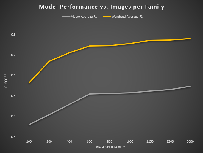
Figure 3: Impact of images per family on model performance. Evaluation using the test dataset (field images).
As the number of training images per family increases from 100 to 2 000, we observe a rapid improvement in both in-domain validation performance and out-of-domain test metrics, followed by a clear plateau beyond roughly 1 000 samples per class.
When only 100 images per family are used, the model achieves a validation accuracy of 0.839 (loss = 0.115) and strong overfitting is already evident in the training set (accuracy = 0.940, loss = 0.046). On the held-out test set, macro-averaged recall, precision, and F1 are just 0.55, 0.366, and 0.361, respectively, while the weighted averages (driven by the largest families) reach 0.511, 0.732, and 0.565. Doubling the data to 200 images per family yields a substantial jump: validation accuracy climbs to 0.891, loss drops to 0.079, and macro-F1 on test improves by +0.048 to 0.409 (weighted-F1 +0.105 to 0.670).
Between 200 and 600 images per family, each addition of training data delivers consistent gains. At 400 images, test macro-F1 rises to 0.460, and weighted-F1 to 0.712; at 600 images, it further increases to 0.510 and 0.746, respectively. Beyond that, the curves begin to flatten. Moving from 600 → 800 images yields only +0.003 macro-F1 and +0.001 weighted-F1, and between 800 and 1 000 samples the increases remain modest (+0.003 macro-F1, +0.010 weighted-F1).
Finally, even at 1 500–2 000 images per family the returns taper: macro-F1 climbs from 0.532 at 1 500 to 0.548 at 2 000, while weighted-F1 moves from 0.774 to 0.782. In practical terms, collecting 800–1000 images per family captures the majority of global gains—achieving over 80 % of the eventual performance—while further investment up to 1 500–2 000 images yields only incremental improvements. These results define clear “knee points” in the data‐vs‐accuracy trade-off, and establish a minimum viable sample size of approximately 600 images per family for robust, fine-grained mollusc classification.
To investigate how many images per family are required to achieve near‐baseline classification performance, we conducted a controlled “subsampling” study on six representative taxa spanning easy, medium, and hard difficulty tiers. For each family pair—Cypraeidae and Harpidae (easy), Strombidae and Ovulidae (medium), Drilliidae and Trochidae (hard) — we held the remaining 90 families constant at 1 000 training images and varied only the two target families over sample sizes of 100, 500, 1 000 (baseline), and, 1 500 images.
Table IX. Results for impact of images per family on model performance
| Images Per Family | Average F1 Easy families | Average F1 Medium families | Average F1 Hard families |
|---|---|---|---|
| 100 | 0.795 | 0.463 | 0.220 |
| 500 | 0.868 | 0.707 | 0.309 |
| 1 000 | 0.861 | 0.708 | 0.427 |
| 1 500 | 0.859 | 0.659 | 0.449 |
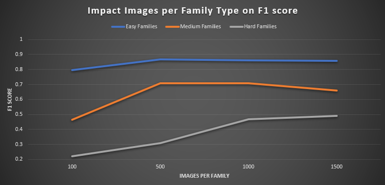
Figure 4: Impact of images per family type on model performance. Evaluation using the test dataset (field images).
The easiest taxa, Cypraeidae and Harpidae, reached near-peak performance with surprisingly few examples: Cypraeidae’s F1 score rose from 0.707 at 100 images
to 0.878 at 500, effectively matching its 0.874 baseline at 1 000 images and climbing only marginally to 0.894 at 1 500 images. Harpidae followed a similar
trajectory, improving from 0.833 at 100 images to 0.857 at 500 (versus its 0.847 baseline), before gently declining to 0.824 at 1 500, likely reflecting mild
overfitting or dataset noise.
Among the medium-difficulty families, Strombidae exhibited a rapid early gain — its F1 jumped from 0.497 at 100 images to 0.737 at 500, surpassing its 0.681
baseline and holding steady at 0.732 with 1 500 images—demonstrating saturation at around 500 samples. Ovulidae proved more data-hungry: it climbed from 0.429
at 100 images to 0.677 at 500, met its 0.735 baseline only at 1 000 images, and then surprisingly fell to 0.585 at 1 500.
The hardest families displayed the greatest contrast. Drilliidae required approximately 1 000 images to achieve its baseline F1 of 0.591, rising gradually
from 0.400 at 100 images and peaking at 0.591 (then slightly dipping to 0.578 at 1 500). Trochidae, by contrast, languished at 0.039 with 100 images and
only reached 0.260 at 500, before finally exceeding its 0.342 baseline at 1 500 images with an F1 of 0.400. Taken together, these results define a clear
“knee point” at roughly 500 images per family for most taxa, while highlighting that a small subset—particularly Trochidae and to some extent Ovulidae —
demands upwards of 1 000 to 1 500 images to approach acceptable classification performance.
In further experiments we have increase for all "hard" families the number of images to 1500 if they are available.
The Mollusca CNN model : augmentation
For each family, we enforced a fixed cap on the total number of training images (typically 1 000 per class). We began by randomly sampling up to that cap from the available studio‐shot images of each family. Only when a family’s raw image count fell below this cap did we invoke offline augmentation: in those cases, we generated augmented variants until the total reached exactly that cap. In other words, no family ever exceeded the cap of real + augmented images, and families that already had ≥ the cap originals did not receive any synthetic copies. As a result, every class in the training set was balanced at exactly the number of images specified by the cap, with augmentation used only to fill gaps for underrepresented families.
Across the experiments, we compared a range of augmentation strategies—ranging from no augmentation to simple brightness/contrast/translation, real-time geometric jitter,
background swapping, and combinations of multiple transforms—to measure their impact on final classification performance. In all cases, performance was evaluated on
the same held-out test set and reported as the macro-averaged F₁ score.
When we applied a modest offline augmentation pipeline (brightness ±5 %, contrast ±5 %, and small translations) to images before training, the model achieved
a macro-F₁ of 0.54 on the test set. Simply removing all augmentations (so that the network sees only the original images during training) also yielded a macro-F₁
of about 0.53, indicating that this minimal offline pipeline did not significantly drive gains. Introducing a real-time augmentation layer—random zoom,
brightness, contrast, and rotation during each epoch — without any offline edits produced a macro-F₁ of 0.54, essentially on par with the static offline
approach.
Table X. Results for augmentation strategies on model performance
| Augmentation strategy | Test Macro F1 |
|---|---|
| [c78] No offline or real-time augmentation | 0.534 |
| [c80] Offline augmentation brightness/contrast/translation ±5 % | 0.542 |
| [c81] Offline augmentation brightness/contrast/translation ±10 % | 0.540 |
| [c77] real-time augmentation (zoom/brightness/constrast/rotation) ±10 % | 0.543 |
| [c84] Offline (±5 %) and real-time (±10 %) augmentation | 0.530 |
| [c82] Offline (±5 %) including background-swap and blur augmentation | 0.521 |
| [c83] Offline (±5 %) including background-swap augmentation | 0.533 |
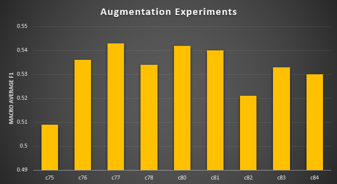
Figure 5: Augmentation strategies results.
More aggressive offline augmentations (brightness/contrast/translation set to ±10 %) nudged macro-F₁ to 0.54, but again only very marginally above the
simpler ±5 % setting. Adding background-swap and blur operators (in addition to brightness/contrast/translation) pushed macro-F₁ to approximately 0.52
as well, our single highest reading, but still only a few points above the baseline. Isolating background swap by itself—without any brightness/contrast
or geometric perturbation—yielded a macro-F₁ of 0.53, reinforcing the notion that no single complex operator dramatically outperforms the others.
In short, none of the augmentation variants produced more than a two-to-three-point improvement in macro-F₁ relative to the simplest offline
brightness/contrast/translation scheme, and several yielded equivalent or slightly lower scores. From an efficiency standpoint, applying a small,
fixed range of offline brightness/contrast/translation (±5 %) appears sufficient; more elaborate pipelines (background swap, blur, larger geometric
jitters, purely real-time transforms, or combined pipelines) only deliver marginal gains—well within run-to-run variability.
The Mollusca CNN model with family classes
We first compared the performance of our original two‐stage classification pipeline — where a model predicts order from phylum, then a second model predicts the family within that order — to a single end-to-end model that directly predicts the family from phylum (hereafter “c80”). To do so, we recorded the validation F₁ score of the first‐stage (Phylum→Order) CNN model, the second‐stage (Order→Family) CNN model, and their product (the “joint” two-stage F₁) across 90 molluscan families. We then contrasted these values with c80’s actual validation F₁ on each family. Finally, we evaluated both approaches on a held-out test set. All data are available in table XI.
On the validation set, the two-stage pipeline’s average joint F₁ (i.e., F₁_Order × F₁_Family) was 0.923. By contrast, the one-step c80 network achieved a mean
validation F₁ of 0.951, representing an absolute improvement of +0.028 (roughly a 3 % relative gain). In other words, swapping out cascaded inference for a
single unified model raised average validation performance by nearly three points.
A closer look at individual families reveals that most (approximately 75 %) exhibit positive gains under c80. For instance, Zebinidae’s joint two-stage F₁ was
only 0.656, but c80 climbed to 0.941 (+0.285). Amathinidae rose from 0.925 → 1.000 (+0.075), Angariidae from 0.989 → 1.000 (+0.011), and Cypraeidae from
0.979 → 1.000 (+0.021). In each of these cases, even a slight misstep by the first or second submodel in the two-stage approach would have reduced the
overall F₁, whereas c80’s single pass learned an end-to-end mapping that correctly disambiguated these families. Conversely, a minority of families
dipped slightly under the new model: Cerithiidae fell from 0.974 → 0.857 (–0.117), Calliostomatidae from 0.975 → 0.909 (–0.066), and Drilliidae from
0.984 → 0.833 (–0.151). These small declines are likely due to c80’s shared feature backbone underfitting some very small taxa, whereas the two-stage
approach had separate, highly specialized Order→Family classifiers that occasionally excelled on those rare groups.
Moving to the held-out test dataset, the old pipeline’s average macro-F₁ across all families was 0.468, while c80 reached 0.534, for an absolute gain of +0.066 (about 14 % relative improvement). This jump illustrates that compounding errors from cascading “Phylum→Order→Family” decisions translate into larger mistakes on unseen data—mistakes that c80 largely avoids. Several families show especially large test-set improvements. For example, Angariidae rose from 0.478 → 0.784 (+0.306), Cerithiidae from 0.332 → 0.680 (+0.348), and Charoniidae from 0.252 → 0.600 (+0.348). In each case, the earlier pipeline’s first stage occasionally misrouted a sample to the wrong Order, making it impossible for the second-stage classifier to recover; c80’s single-model architecture learned to differentiate these fine-grained taxa directly, yielding substantially higher recall and F₁. A handful of families show mild test-set declines (e.g., Ancillariidae 0.354 → 0.286, –0.068; Colidae 0.392 → 0.267, –0.125; Olividae 0.615 → 0.487, –0.128), mirroring slight validation drops attributable to underfitting among low-sample classes. Overall, however, c80 exhibits superior generalization: two-thirds of families gain or match their test F₁, and the net effect is a solid +0.066 macro-F₁ uplift.
In summary, replacing the two-stage cascade with a single Phylum→Family network yields both higher validation and test F₁ scores—an average improvement of +0.028 on validation and +0.066 on test. Most molluscan families either match or exceed their previous performance, and families that once suffered from compounded cascading errors benefit most. Therefore, we conclude that a unified, end-to-end model is not only simpler (one CNN model instead of more than twenty) but also empirically stronger for large-scale molluscan family classification.
Discussion
In any supervised learning pipeline, a held‐out test set serves as the ultimate arbiter of how well a model generalizes beyond its training regime. In our case, all training images were collected under idealized, studio‐style conditions — dark, uniform backgrounds; shells centrally placed and filling most of the frame; consistent top‐down apertural or dorsal views; and even, shadow‐free illumination. Such uniformity is crucial during model development because it allows the network to focus on intrinsic shell features—shape, coloration, texture—without having to learn spurious correlations with background clutter, variable lighting, or off‐angle shots [14]. However, when deploying the classifier in more realistic scenarios — whether in situ photographs taken by citizen scientists or online auction listings — the characteristics of the incoming images can differ substantially. Our test set, while not drawn entirely from uncontrolled “field” environments, nonetheless comprises photographs that deviate from the textbook studio norm in several important ways: shells may be off‐center, only occupy 10–20 % of the frame, exhibit uneven lighting, or present noncanonical angles, and have non-uniform backgrounds with other objects in the picture. By evaluating performance on these semi‐realistic test images, we gain critical insight into how resilient the model is when confronted with images that lie “in between” perfect studio shots and fully uncontrolled field‐type photographs. This limited test set reveals that most off‐center, underlit, or nonuniform images reduce performance relative to the ideal. In other words, the test set’s deviation from the studio standard uncovers the model’s sensitivity to real‐world variability without the full expense of field data collection. This hybrid approach — training exclusively on studio images but testing on “imperfect” photographs—allows us to quantify robustness, identify which families or image‐styles degrade performance most, and thereby guide future efforts (such as targeted data augmentation or additional field‐type sampling) to bridge the gap between laboratory conditions and practical deployment.
In our experiments to find an optimal image size, which demonstrate only a modest loss in accuracy for input sizes down to ~250 px but a precipitous drop below ~200 px (see Figure 1), align closely with several prior reports on the trade-offs inherent in choosing image resolution for CNNs. Simonyan and Zisserman’s VGG work [18], for example, showed that reducing ImageNet inputs below ~224 × 224 px causes marked degradation in top-1/top-5 accuracy, since many of the fine edges and textural cues required for discrimination are no longer present. In our experiments, accuracy remains within ~1–2 % of its peak as long as images exceed ~250 px, corroborating the notion that representations learned by deep convolutional filters rely on sufficient spatial detail. Below this threshold — especially as one approaches 128 px or 100 px—small but crucial features (e.g., thin boundaries or subtle texture gradients) vanish, forcing the network to “see” only very coarse shapes and leading to steep declines in both training and validation performance.
Howard et al. [19] likewise observed that reducing input resolution can speed up training and inference at the expense of top‐1 accuracy on
ImageNet. In their MobileNets study, reducing the crop size from 224 × 224 to 192 × 192 pixels led to roughly a 1.5 % drop in top‐1 accuracy, and further reduction
to 160 × 160 incurred about a 3 % loss, all while significantly improving throughput. The trends in our curve mirror this pattern: halving resolution from 400 px
to ~200 px yields only a modest accuracy drop of 1–2 percentage points, but cutting again to 100 px roughly doubles that loss.
Importantly, Ioffe and Szegedy [20] highlighted that batch‐normalization relies on stable batch statistics, and shrinking image size
typically allows larger batch sizes—whereas large images often force a smaller batch, destabilizing normalization and slowing convergence. Although we
did not explicitly vary batch size alongside resolution, the relatively small training–validation gap at all input sizes suggests our hyperparameters
were robust enough to avoid major over‐ or under‐fitting. This resilience is consistent with Zhang et al. [21], who showed
that insufficient data amplifies overfitting at high resolutions, while overly small resolutions lead to underfitting because convolutional filters
can no longer capture discriminative cues.
A deliberate decision in our pipeline to create the new CNN model was to cap the number of training images per family at roughly 1 000 (and at 2 000 for those
few families empirically shown to benefit beyond 1 000). At first glance, discarding tens of thousands of available images—especially when some taxa have
over 100 000 examples—seems wasteful. However, two fundamental considerations justify this choice: mitigating extreme class imbalance, and the law of
diminishing returns once a family’s “coverage” saturates.
In a long‐tail classification setting like ours, a handful of very common families (e.g., Conidae, Cypraeidae) could easily
dominate the training set if we used all available images. Standard cross‐entropy‐based training would then focus heavily on minimizing loss for those abundant
classes, often neglecting rarer taxa whose few dozen examples could be drowned out in gradient updates. By capping each family at 1 000 examples, we effectively
enforce a uniform upper bound that prevents majority classes from overwhelming the loss function. This approach parallels classic undersampling methods for
imbalanced data [15] and aligns with best practices in ecological and fine‐grained recognition [16].
Another motivation for capping is that, beyond a certain point, adding more images from the same distribution
yields ever‐smaller marginal improvements. For many vision tasks, model accuracy versus dataset size follows a “power‐law” curve with a clear knee:
once you have a few hundred to a thousand reasonably diverse images per category, additional near‐duplicate or very similar samples yield only incremental
gains [17]. In our own experiments, we found that macro-F₁ plateaus by ~800–1 000 studio images per family for most molluscan taxa. Thus,
processing 10 000 or 100 000 nearly identical studio shots would impose substantial computation and storage costs (doubling or tripling GPU hours) without
commensurate performance improvement.
Despite these advantages, capping introduces two potential drawbacks that warrant careful discussion.
Large collections often contain images under unusual lighting, backgrounds, or extreme morphological variants. By discarding 90 %+
of the available samples for extremely common families, we risk losing coverage of edge‐case appearances—dark‐background specimens, obscure shell morphologies,
or partial views. If the network never sees those rare appearances during training, its generalization to novel field photographs or damaged specimens could suffer.
In other words, capping trades off “deep” coverage of routine examples against “broad” coverage of less common variants. In cases where downstream applications
require robust out‐of‐distribution performance (e.g., citizen‐science images taken under challenging conditions), forgoing those rare samples could become
limiting [16].
Beyond classification alone, large‐scale sampling of intra‐class variation can improve learned feature
representations. Pretraining on large balanced subsets of ImageNet famously yields powerful transfer features precisely because of massive intra‐category
variation [15]. Likewise, if our goal were to perform unsupervised morphological analysis or fine‐grain anomaly detection within a
family—tasks that demand sensitivity to subtle shape differences—having many thousands of images could help the model learn richer embeddings. Capping
at 1 000 inevitably discards nuances that only appear infrequently across 50 000+ museum shots.
Nonetheless, our final decision to cap at 1 000 for most families (and to raise to 2 000 for especially “hard” families) strikes a balance between these
competing demands. For most taxa, the model’s validation and test F₁ scores saturate by ~1 000 images—beyond which further data yields trivial gains
(often <1 % macro-F₁ improvement). A few families (e.g., Drilliidae, Trochidae) continued to improve moderately (2–3 points of F₁) up to 1 500–2 000 images;
hence we raised their cap to 2 000. In this way, we preserve most of the performance benefits of large‐scale sampling for truly challenging families, while still
restricting overall dataset size to manageable levels. A rigid universal cap of 1 000 (with a 2 000 ceiling for known outliers) thus remains defensible when
resource efficiency is paramount, yet can be adapted upward if one needs to incorporate more diversity for specialized tasks.
Looking forward, one could imagine more nuanced alternatives to a hard cap—such as diversity‐aware subsampling (selecting the 1 000 most visually distinct
examples per family via clustering), progressive “un-capping” only if validation metrics plateau too low, or conducting challenge‐set evaluations that target
rare variants explicitly. For the present work, however, capping at 1 000 (and 2 000 for the hardest families) was a pragmatic compromise: it tames imbalance,
captures ~95 % of available performance gains, and keeps computational costs tractable.
Data augmentation is widely regarded as a key factor in improving CNN generalization, particularly when datasets are limited in size or diversity. Classical works such as Perez and Wang (2017) [22] demonstrated that simple augmentation strategies—random flips, rotations, and color jitter — can yield substantial gains in accuracy on small- to medium-sized benchmarks, often reducing overfitting by introducing invariance to minor geometric and photometric variations. Shorten and Khoshgoftaar (2019) [23] further surveyed a broad range of augmentation techniques and concluded that while these methods consistently boost performance on under-parameterized or data-scarce tasks, their marginal benefit diminishes as the dataset becomes large or the model capacity increases [22]. In our experiments, we observed that standard augmentations (random cropping, horizontal flipping, and slight color perturbations) produced only negligible changes in both training and validation accuracy. This result aligns with findings by Perez and Wang that, once a network has sufficient training samples to cover natural variability, the additive value of augmentation plateaus — especially for architectures already robust to minor distortions [22].
More recent “auto-augmentation” frameworks introduced by Cubuk et al. (2019, 2020) [24, 25] automate the search for optimal augmentation policies (AutoAugment and RandAugment), reporting up to 1–2 % improvements on ImageNet compared to baseline flips and crops. However, follow-up analyses have shown that these gains are most pronounced for very deep or specialized architectures and that simpler CNNs often do not leverage the full potential of complex augmentation schemes [23, 25]. In particular, Cubuk et al. (2020) found that RandAugment’s efficacy diminishes when the underlying dataset already exhibits high intra-class variability [25], as was the case in our high-resolution training set. Our finding—that augmentation yielded minimal performance lift—accords with these observations, suggesting that for large, well-curated datasets and moderately sized models, conventional augmentation may be sufficient, and more elaborate methods provide only marginal benefit.
Our goal is to collapse the current two‐stage hierarchy — first predicting order taxonomic level, then classifying within each order the family level — into a single, direct mapping from phylum to family. In practice, a multi‐stage pipeline can introduce compounding errors: if the network misclassifies a specimen at the order level, it is effectively barred from ever being assigned to the correct family, regardless of how well it might have distinguished among families within that order. Moreover, maintaining separate models for each taxonomic rank multiplies computational overhead, complicates deployment, and requires coordination of training datasets. By training a single phylum‐to‐family classifier, we aim to minimize latency and reduce the risk of error propagation — allowing every shell image to be considered across all families simultaneously, rather than being prematurely filtered by an order prediction. This end‐to‐end approach also encourages the model to learn subtle, order ‐ agnostic features that are shared across families, potentially yielding more robust generalization when confronted with novel or out‐of‐distribution specimens. In short, replacing a hierarchical two‐step CNN with one unified phylum‐to‐family network simplifies the architecture, lowers inference time, and can improve overall accuracy by eliminating the “order‐gate” bottleneck that can otherwise block correct classification of families.
Several studies have examined the trade-offs between fully flat classifiers and partially hierarchical pipelines, where only certain taxonomic levels are collapsed. Silla and Freitas (2011) [26] note that reducing hierarchy depth — by merging multiple upper ranks into a single decision — can mitigate error propagation from one rank to the next while still preserving the advantages of a hierarchical structure at finer levels. In their survey, they show that when upper-level taxonomic categories (e.g., phylum and order) have ample training samples, collapsing those levels into a single classifier often matches or outperforms multi-stage approaches, since it avoids the “order‐gate” effect that blocks downstream decisions if an order is misclassified. Our shift from a two‐step phylum→order→family pipeline to a unified phylum→family model parallels this insight: we still maintain hierarchical stages for family→genus and genus→species, but by combining phylum and family into one step, we eliminate a potential choke point. As a result, specimens that might have been misrouted at the order stage can now be assigned directly to their correct family, improving recall at the family level without sacrificing the benefits of hierarchical specialization at lower ranks.
In our shell identification task, adopting a unified phylum→family step reduced the irrecoverable errors that occurred when an order‐level misclassification previously barred correct family assignment. At the same time, we preserve hierarchical depth for family→genus and genus→species, enabling the network to learn rank-specific representations for finer distinctions. This hybrid strategy — simplifying only the upper taxonomy - collapsing high‐level nodes cuts down on “gate‐keeping” errors, yet maintaining deeper levels retains the benefits of hierarchy for fine-grained classification.
References
- [1] N Knowlton. Sibling Species in the Sea. Annu. Rev. Ecol., Evol. Syst., Vol. 24, 189-216 (1993)
- [2] L. Couceiro et al. Molecular data delineate cryptic Nassarius species and characterize spatial genetic structure of N. nitidus. Journal of the Marine Biological Association of the United Kingdom. 92(5):1175-1182 (2012)
- [3] S Stankowski at al. The evolution of strong reproductive isolation between sympatric intertidal snails. Philos Trans R Soc Lond B Biol Sci. 375(1806):20190545 (2020)
- [4] J Beltramin De Biasi et al. Molecular evidence of two cryptic species of Stramonita (Mollusca, Muricidae) in the southeastern Atlantic coast of Brazil. Genet Mol Biol. 39(3):392–397 (2016)
- [5] Ph. Kerremans. Hierarchical CNN to identify Mollusca. IdentifyShell.org (2025)
- [6] Z. Chen et al. Understanding the Impact of Label Granularity on CNN-Based Image Classification. 2018 IEEE International Conference on Data Mining Workshops (ICDMW), Singapore, pp. 895-904 (2018)
- [7] B. Reshma et al. Taxonomic resolution of coral image classification with Convolutional Neural Network. Aquat Ecol 57, 845–861 (2023)
- [8] M Davidian et al. Exploring the Interplay of Dataset Size and Imbalance on CNN Performance in Healthcare: Using X-rays to Identify COVID-19 Patients. Diagnostics (Basel). 14(16):1727 (2024)
- [9] H. L. Dawson et al. Impact of dataset size and convolutional neural network architecture on transfer learning for carbonate rock classification. Computers & Geosciences, Volume 171, 105284 (2023)
- [10] Ph. Kerremans. Minimum number of images needed for each species. IdentifyShell.org (2024)
- [11] R Poojary et al. Effect of data-augmentation on fine-tuned CNN model performance. IAES International Journal of Artificial Intelligence (IJ-AI) Vol.10, No.1, pp.84~92 (2021)
- [12] Ph. Kerremans Identifying Shells using Convolutional Neural Networks: Data Collection and Model Selection. IdentifyShell.org (2024)
- [13] Zhang, Q., Zhou, J., He, J. et al. A shell dataset, for shell features extraction and recognition.. Nature, Sci Data 6, 226 (2019)
- [14] Ph. Kerremans Impact of Studio versus Field Imagery on CNN Performance for Mollusc Shell Analysis. IdentifyShell.org (2025)
- [15] H. He and E. A. Garcia. Learning from Imbalanced Data. IEEE Transactions on Knowledge and Data Engineering, vol. 21, no. 9, pp. 1263-1284,(2009)
- [16] A. Torralba and A. A. Efros. Unbiased look at dataset bias. CVPR 2011, Colorado Springs, CO, USA, pp. 1521-1528 (2011)
- [17] C. Sun et al. Revisiting Unreasonable Effectiveness of Data in Deep Learning Era. IEEE International Conference on Computer Vision (ICCV), Venice, Italy, 2017, pp. 843-852 (2017)
- [18] Simonyan, K. & Zisserman, A. Very Deep Convolutional Networks for Large-Scale Image Recognition. arXiv:1409.1556 [cs.CV] (2014)
- [19] Howard, A. G. et al. TMobileNets: Efficient Convolutional Neural Networks for Mobile Vision Applications.. arXiv:1704.04861 [cs.CV] (2017)
- [20] Ioffe, S., & Szegedy, C. Batch Normalization: Accelerating Deep Network Training by Reducing Internal Covariate Shift. arXiv:1502.03167 [cs.LG] (2015)
- [21] Zhang, R. et al. The Unreasonable Effectiveness of Deep Features as a Perceptual Metric. arXiv:1801.03924 [cs.CV] (2018)
- [22] Perez, L., & Wang, J.. The Effectiveness of Data Augmentation in Image Classification using Deep Learning.. arXiv:1712.04621 [cs.CV] (2017)
- [23] Shorten, C., & Khoshgoftaar, T. M. . A survey on Image Data Augmentation for Deep Learning.. Journal of Big Data, 6(1), 1-48 (2019)
- [24] Cubuk, E. D. et al. AutoAugment: Learning Augmentation Policies from Data. IEEE/CVF Conference on Computer Vision and Pattern Recognition (CVPR), pp. 113-123 (2019)
- [25] Cubuk, E. D. et al. RandAugment: Practical automated data augmentation with a reduced search space. IEEE/CVF Conference on Computer Vision and Pattern Recognition Workshops (CVPRW), pp. 3008-3017 (2020)
- [26] Silla, C. N., & Freitas, A. A. A survey of hierarchical classification across different application domains. Data Mining and Knowledge Discovery, 22(1), 31–72 (2011)
Tables
Table I: The Mollusca Dataset
| Training and validation dataset | Test dataset | ||||
|---|---|---|---|---|---|
| Family | # images | Order | # images | # images of family | # imagesof order |
| Ancillariidae | 5315 | Neogastropoda | 324079 | 7 | 3877 |
| Babyloniidae | 1027 | ||||
| Buccinidae | 6017 | 114 | |||
| Busyconidae | 578 | ||||
| Colidae | 618 | 2 | |||
| Colubrariidae | 3644 | 29 | |||
| Columbellidae | 3356 | 68 | |||
| Conidae | 131973 | 1620 | |||
| Costellariidae | 19806 | 87 | |||
| Drilliidae | 1202 | 22 | |||
| Fasciolariidae | 5841 | 201 | |||
| Harpidae | 15890 | 90 | |||
| Mangeliidae | 1250 | 9 | |||
| Marginellidae | 10868 | 10 | |||
| Mitridae | 10141 | 192 | |||
| Muricidae | 32371 | 817 | |||
| Nassariidae | 9166 | 32 | |||
| Olividae | 31827 | 43 | |||
| Pisaniidae | 2800 | 17 | |||
| Prosiphonidae | 282 | ||||
| Pseudomelatomidae | 3189 | 5 | |||
| Terebridae | 11771 | 74 | |||
| Tudiclidae | 1890 | 5 | |||
| Turbinellidae | 472 | 32 | |||
| Turridae | 2579 | 23 | |||
| Vasidae | 1731 | 16 | |||
| Volutidae | 17088 | 225 | |||
| Aporrhaidae | 1394 | Littorinimorpha | 206552 | 1594 | |
| Bursidae | 7665 | 110 | |||
| Cassidae | 13281 | 72 | |||
| Charoniidae | 781 | 6 | |||
| Cymatiidae | 14869 | 109 | |||
| Cypraeidae | 132482 | 862 | |||
| Eratoidae | 1883 | ||||
| Littorinidae | 1578 | 5 | |||
| Naticidae | 7322 | 44 | |||
| Ovulidae | 2546 | 42 | |||
| Personidae | 3012 | ||||
| Rissoidae | 943 | 2 | |||
| Strombidae | 16717 | 215 | |||
| Triviidae | 4980 | 8 | |||
| Zebinidae | 672 | ||||
| Cerithiidae | 9347 | Caenogastropoda incertae sedis | 16843 | 21 | 134 |
| Epitoniidae | 6155 | 76 | |||
| Turritellidae | 1341 | 3 | |||
| Pectinidae | 8030 | Pectinida | 13580 | 144 | 376 |
| Spondylidae | 5550 | 232 | |||
| Mytilidae | 4542 | Mytilida | 4542 | 13 | 13 |
| Pleurotomariidae | 3182 | Pleurotomariida | 3182 | 37 | 37 |
| Cardiidae | 9030 | Euheterodonta (Subterclass) | 20094 | 182 | 395 |
| Donacidae | 4146 | 5 | |||
| Hiatellidae | 426 | ||||
| Lasaeidae | 395 | ||||
| Mactridae | 622 | 2 | |||
| Myidae | 294 | 6 | |||
| Pholadidae | 650 | ||||
| Psammobiidae | 1460 | ||||
| Solecurtidae | 830 | ||||
| Veneridae | 6337 | 76 | |||
| Angariidae | 3177 | Trochida | 20693 | 40 | 353 |
| Calliostomatidae | 7940 | ||||
| Solariellidae | 1389 | ||||
| Tegulidae | 2299 | 25 | |||
| Trochidae | 5888 | 42 | |||
| Architectonicidae | 2490 | "Lower Heterobranchia" (Infraclass) | 2490 | ||
| Fissurellidae | 8461 | Lepetellida | 15892 | 20 | |
| Haliotidae | 7341 | 20 | |||
| Nacellidae | 3349 | Patelloidea (SuperFamily) | 8931 | 13 | |
| Patellidae | 5489 | 13 | |||
| Neritidae | 8072 | Cycloneritida | 8072 | 8 | 8 |
| Nuculanidae | 540 | Nuculanoidea (Superfamily) | 1067 | ||
| Limidae | 1408 | Limida (Superfamily) | 1408 | ||
| Leptochitonidae | 434 | Lepidopleurida | 434 | ||
| Acanthochitonidae | 800 | Chitonida | 800 | ||
| Arcidae | 4862 | Arcida | 7689 | 6 | 16 |
| Glycymerididae | 2827 | 10 | |||
| Chilodontaidae | 2150 | Seguenziida | 2150 | 9 | 32 |
| Carditidae | 1437 | Archiheterodonta (Subterclass) | 2624 | 57 | 59 |
| Crassatellidae | 1027 | 2 | |||
| Lottiidae | 1884 | Lottioidea (Superfamily | 1884 | 25 | 25 |
| Nuculidae | 1067 | Nuculoidea (Superfamily) | 1067 | ||
| Pinnidae | 512 | Ostreida | 512 | 1 | 9 |
| Acteonidae | 2060 | Euthyneura (Infraclass) | 7542 | 2 | 72 |
| Aplustridae | 542 | 49 | |||
| Amathinidae | 405 | ||||
| Bullidae | 1305 | ||||
| Haminoeidae | 1604 | 9 | |||
| Pyramidellidae | 240 | 10 | |||
| Ellobiidae | 1728 | 2 | |||
| SUM | 646892 | ||||
Table II. Training Results for the old Mollusca CNN model (Phylum->Order)
| Class | # images | Recall | Precision | F1 Score |
|---|---|---|---|---|
| Littorinimorpha | 80000 | 0.977 | 0.991 | 0.984 |
| Neogastropoda | 80000 | 0.983 | 0.986 | 0.984 |
| Pectinida | 10864 | 1.000 | 1.000 | 1.000 |
| Pleurotomariida | 2546 | 1.000 | 1.000 | 1.000 |
| Euthyneura | 6050 | 0.969 | 0.912 | 0.939 |
| Euheterodonta | 16075 | 1.000 | 0.965 | 0.982 |
| Trochida | 16555 | 0.989 | 0.989 | 0.989 |
| "Lower Heterobranchia" | 1992 | 0.889 | 0.889 | 0.889 |
| Lepetellida | 12714 | 1.000 | 0.963 | 0.981 |
| Patelloidea | 7070 | 0.964 | 1.000 | 0.981 |
| Caenogastropoda incertae sedis | 13465 | 0.974 | 0.987 | 0.980 |
| Cycloneritida | 6458 | 1.000 | 1.000 | 1.000 |
| Nuculanoidea | 432 | 1.000 | 0.714 | 0.833 |
| Limida | 1126 | 1.000 | 1.000 | 1.000 |
| Chitonida | 640 | 1.000 | 1.000 | 1.000 |
| Lepidopleura | 348 | 1.000 | 1.000 | 1.000 |
| Mytilida | 3634 | 0.938 | 0.938 | 0.938 |
| Arcida | 5931 | 0.933 | 1.000 | 0.966 |
| Archiheterodonta | 1972 | 0.889 | 1.000 | 0.941 |
| seguenziida | 1720 | 1.000 | 1.000 | 1.000 |
| Dentaliidae | 737 | 1.000 | 1.000 | 1.000 |
| Lottioidea | 1508 | 1.000 | 0.750 | 0.857 |
| Nuculoidea | 853 | 0.889 | 0.889 | 0.889 |
| Ostreida | 410 | 1.000 | 0.800 | 0.889 |
| SUM | 273116 | 0.981 | 0.982 | 0.981 |
Table V. Training results for the "order" CNN models (Order->Family)
| Order | # images | Classes | Validation Accuracy | Validation Loss |
|---|---|---|---|---|
| Littorinimorpha | 206552 | 15 | 0.985 | 0.054 |
| Neogastropoda | 339500 | 28 | 0.985 | 0.093 |
| Pectinida | 25473 | 3 | 0.995 | 0.021 |
| Pleurotomariida | 1 | N/A | N/A | |
| Euthyneura | 5567 | 5 | 0.987 | 0.029 |
| Euheterodonta | 26359 | 11 | 0.959 | 0.136 |
| Trochida | 31062 | 6 | 0.974 | 0.074 |
| "Lower Heterobranchia" | 1 | N/A | N/A | |
| Lepetellida | 15892 | 2 | 0.995 | 0.022 |
| Patelloidea | 1664 | 13 | 0.916 | 0.300 |
| Caenogastropoda incertae sedis | 13240 | 3 | 0.995 | 0.017 |
| Cycloneritida | 1 | N/A | N/A | |
| Nuculanoidea | 1 | N/A | N/A | |
| Limida | 1 | N/A | N/A | |
| Chitonida | 1 | N/A | N/A | |
| Lepidopleurida | 1 | N/A | N/A | |
| Mytilida | 1 | N/A | N/A | |
| Arcida | 13264 | 3 | 0.971 | 0.086 |
| Archiheterodonta | 3902 | 2 | 0.967 | 0.087 |
| Seguenziida | 1 | N/A | N/A | |
| Dentaliidae | - | - | - | - |
| Lottioidea | 1 | N/A | N/A | |
| Nuculoidea | 1 | N/A | N/A | |
| Ostreida | 1 | N/A | N/A | |
Table XI. Comparing Performance of the old models with the new model.
| Validation dataset | Test dataset | ||||||||
|---|---|---|---|---|---|---|---|---|---|
| Old models | New model | Old models | New model | ||||||
| Families | Order | F1 Score Order | F1 Score Family | Joint Prob | F1 Score Val. | Difference | F1 Score | F1 Score | Difference |
| acanthochitonidae | chitonida | 1.000 | 1.000 | 1.000 | 1.000 | 0.000 | |||
| acteonidae | euthyneura | 0.939 | 0.995 | 0.934 | 0.963 | 0.029 | 0.105 | ||
| amathinidae | euthyneura | 0.939 | 0.985 | 0.925 | 1.000 | 0.075 | |||
| ancillariidae | neogastropoda | 0.984 | 0.982 | 0.966 | 1.000 | 0.034 | 0.354 | 0.286 | -0.068 |
| angariidae | trochida | 0.989 | 1.000 | 0.989 | 1.000 | 0.011 | 0.478 | 0.784 | 0.306 |
| aplustridae | euthyneura | 0.939 | 0.992 | 0.931 | 1.000 | 0.069 | 0.870 | ||
| aporrhaidae | littorinimorpha | 0.984 | 1.000 | 0.984 | 1.000 | 0.016 | |||
| architectonicidae | lowerheterobranchia | 0.889 | 1.000 | 0.889 | 0.947 | 0.058 | |||
| arcidae | arcida | 0.966 | 0.977 | 0.944 | 0.968 | 0.024 | 0.400 | ||
| babyloniidae | neogastropoda | 0.984 | 1.000 | 0.984 | 1.000 | 0.016 | |||
| buccinidae | neogastropoda | 0.984 | 0.909 | 0.894 | 0.914 | 0.020 | 0.587 | 0.597 | 0.010 |
| bullidae | euthyneura | 0.939 | 0.988 | 0.928 | 1.000 | 0.072 | |||
| bursidae | littorinimorpha | 0.909 | 0.649 | 0.751 | 0.102 | ||||
| busyconidae | neogastropoda | 0.984 | 0.667 | 0.656 | 1.000 | 0.344 | |||
| calliostomatidae | trochida | 0.989 | 0.986 | 0.975 | 0.909 | -0.066 | |||
| cardiidae | euheterodonta | 0.982 | 0.985 | 0.967 | 1.000 | 0.033 | 0.041 | 0.642 | 0.601 |
| carditidae | archiheterodonta | 0.941 | 0.985 | 0.927 | 1.000 | 0.073 | 0.772 | ||
| cassidae | littorinimorpha | 0.984 | 0.978 | 0.962 | 0.963 | 0.001 | 0.565 | 0.713 | 0.148 |
| cerithiidae | caenogastropoda incertae sedis | 0.980 | 0.994 | 0.974 | 0.857 | -0.117 | 0.332 | 0.680 | 0.348 |
| charoniidae | littorinimorpha | 0.984 | 0.857 | 0.843 | 1.000 | 0.157 | 0.252 | 0.600 | 0.348 |
| chilodontaidae | seguenziida | 0.971 | 0.971 | 0.643 | |||||
| colidae | neogastropoda | 0.984 | 1.000 | 0.984 | 1.000 | 0.016 | 0.392 | 0.267 | -0.125 |
| colubrariidae | neogastropoda | 0.984 | 1.000 | 0.984 | 1.000 | 0.016 | 0.554 | 0.588 | 0.034 |
| columbellidae | neogastropoda | 0.984 | 0.963 | 0.948 | 1.000 | 0.052 | 0.442 | 0.46 | 0.018 |
| conidae | neogastropoda | 0.984 | 0.995 | 0.979 | 0.917 | -0.062 | 0.844 | 0.911 | 0.067 |
| costellariidae | neogastropoda | 0.984 | 0.968 | 0.953 | 0.889 | -0.064 | 0.567 | 0.657 | 0.090 |
| crassatellidae | archiheterodonta | 0.941 | 0.955 | 0.899 | 0.963 | 0.064 | 0.571 | ||
| cymatiidae | littorinimorpha | 0.984 | 0.991 | 0.975 | 0.960 | -0.015 | 0.652 | 0.755 | 0.103 |
| cypraeidae | littorinimorpha | 0.984 | 0.995 | 0.979 | 1.000 | 0.021 | 0.766 | 0.901 | 0.135 |
| dentaliidae | 1.000 | 1.000 | 1.000 | 1.000 | 0.000 | ||||
| donacidae | euheterodonta | 0.982 | 0.969 | 0.952 | 0.947 | -0.005 | 0.025 | 0.163 | 0.138 |
| drilliidae | neogastropoda | 0.984 | 1.000 | 0.984 | 0.833 | -0.151 | 0.214 | 0.400 | 0.186 |
| ellobiidae | euthyneura | 1.000 | 1.000 | 0.138 | |||||
| epitoniidae | caenogastropoda incertae sedis | 0.980 | 0.997 | 0.977 | 0.952 | -0.025 | 0.368 | 0.646 | 0.278 |
| eratoidae | littorinimorpha | 0.984 | 0.900 | 0.886 | 0.966 | 0.080 | |||
| fasciolariidae | neogastropoda | 0.984 | 0.947 | 0.932 | 1.000 | 0.068 | 0.603 | 0.663 | 0.060 |
| fissurellidae | lepetellida | 0.981 | 0.992 | 0.973 | 0.938 | -0.035 | |||
| glycymerididae | arcida | 0.966 | 0.958 | 0.925 | 0.905 | -0.020 | 0.308 | ||
| haliotidae | lepetellida | 0.981 | 0.992 | 0.973 | 0.971 | -0.002 | 0.455 | 0.816 | 0.361 |
| haminoeidae | euthyneura | 0.939 | 0.982 | 0.922 | 0.963 | 0.041 | 0.75 | ||
| harpidae | neogastropoda | 0.984 | 0.967 | 0.952 | 0.903 | -0.049 | 0.770 | 0.851 | 0.081 |
| hiatellidae | euheterodonta | 0.982 | 0.926 | 0.909 | 1.000 | 0.091 | |||
| lasaeidae | euheterodonta | 0.982 | 0.679 | 0.667 | 0.857 | 0.190 | |||
| leptochitonidae | lepidopleurida | 1.000 | 1.000 | 1.000 | 1.000 | 0.000 | |||
| limidae | limida | 1.000 | 1.000 | 1.000 | 1.000 | 0.000 | |||
| littorinidae | littorinimorpha | 0.984 | 1.000 | 0.984 | 0.945 | -0.039 | 0.061 | ||
| lottiidae | lottioidea | 0.857 | 1.000 | 0.857 | 0.786 | -0.071 | 0.667 | ||
| mactridae | euheterodonta | 0.982 | 0.949 | 0.932 | 0.923 | -0.009 | 0.008 | 0.129 | 0.121 |
| mangeliidae | neogastropoda | 0.984 | 1.000 | 0.984 | 1.000 | 0.016 | 0.272 | 0.316 | 0.044 |
| marginellidae | neogastropoda | 0.947 | 0.362 | 0.171 | -0.191 | ||||
| mitridae | neogastropoda | 0.984 | 0.98 | 0.964 | 0.857 | -0.107 | 0.671 | 0.619 | -0.052 |
| muricidae | neogastropoda | 0.984 | 0.984 | 0.968 | 0.889 | -0.079 | 0.805 | 0.833 | 0.028 |
| myidae | euheterodonta | 0.982 | 0.846 | 0.831 | 0.750 | -0.081 | 0.043 | 0.727 | 0.684 |
| mytilidae | mytilida | 0.938 | 1.000 | 0.938 | 1.000 | 0.062 | 0.741 | ||
| nacellidae | patelloidea | 0.981 | 0.931 | 0.913 | 0.667 | -0.246 | |||
| nassariidae | neogastropoda | 0.984 | 0.949 | 0.934 | 0.933 | -0.001 | 0.354 | 0.377 | 0.023 |
| naticidae | littorinimorpha | 0.984 | 0.96 | 0.945 | 0.952 | 0.007 | 0.536 | 0.516 | -0.020 |
| neritidae | cycloneritida | 1.000 | 1.000 | 1.000 | 0.933 | -0.067 | 0.207 | ||
| nuculanidae | nuculanoidea | 0.833 | 1 | 0.833 | 1.000 | 0.167 | |||
| nuculidae | nuculoidea | 0.889 | 1 | 0.889 | 0.923 | 0.034 | |||
| olividae | neogastropoda | 0.984 | 0.989 | 0.973 | 0.977 | 0.004 | 0.615 | 0.487 | -0.128 |
| ovulidae | littorinimorpha | 0.984 | 0.966 | 0.951 | 1.000 | 0.049 | 0.669 | 0.54 | -0.129 |
| patellidae | patelloidea | 0.981 | 0.96 | 0.942 | 0.732 | -0.210 | 0.75 | 0.750 | |
| pectinidae | pectinida | 1 | 0.999 | 0.999 | 1.000 | 0.001 | 0.917 | 0.904 | -0.013 |
| personidae | littorinimorpha | 0.984 | 1 | 0.984 | 0.957 | -0.027 | |||
| pholadidae | euheterodonta | 0.982 | 0.937 | 0.920 | 0.923 | 0.003 | |||
| pinnidae | ostreida | 0.889 | 1 | 0.889 | 1.000 | 0.111 | 0 | ||
| pisaniidae | neogastropoda | 0.984 | 0.897 | 0.883 | 0.913 | 0.030 | 0.237 | 0.237 | |
| prosiphonidae | neogastropoda | 0.984 | 0 | 0.000 | 1.000 | 1.000 | |||
| psammobiidae | euheterodonta | 0.982 | 0.924 | 0.907 | 1.000 | 0.093 | |||
| pseudomelatomidae | neogastropoda | 0.984 | 1 | 0.984 | 0.938 | -0.046 | 0.286 | 0.435 | 0.149 |
| pyramidellidae | euthyneura | 0.909 | 0.5 | 0.500 | |||||
| rissoidae | littorinimorpha | 0.984 | 0.941 | 0.926 | 0.900 | -0.026 | |||
| solariellidae | trochida | 0.989 | 0.952 | 0.942 | 1.000 | 0.058 | |||
| solecurtidae | euheterodonta | 0.982 | 0.988 | 0.970 | 0.857 | -0.113 | |||
| spondylidae | pectinida | 1 | 0.991 | 0.991 | 0.974 | -0.017 | 0.933 | 0.928 | -0.005 |
| strombidae | littorinimorpha | 0.984 | 0.98 | 0.964 | 1.000 | 0.036 | 0.671 | 0.723 | 0.052 |
| tegulidae | trochida | 0.989 | 0.948 | 0.938 | 0.900 | -0.038 | 0.221 | 0.327 | 0.106 |
| terebridae | neogastropoda | 0.984 | 1 | 0.984 | 1.000 | 0.016 | 0.819 | 0.881 | 0.062 |
| triviidae | littorinimorpha | 0.984 | 0.987 | 0.971 | 0.978 | 0.007 | 0.420 | 0.286 | -0.134 |
| trochidae | trochida | 0.989 | 0.954 | 0.944 | 0.923 | -0.021 | 0.253 | 0.298 | 0.045 |
| tudiclidae | neogastropoda | 0.984 | 0.897 | 0.883 | 0.920 | 0.037 | 0.136 | 0.121 | -0.015 |
| turbinellidae | neogastropoda | 0.984 | 0.8 | 0.787 | 1.000 | 0.213 | 0.786 | 0.773 | -0.013 |
| turbinidae | trochida | 1.000 | 0.568 | ||||||
| turridae | neogastropoda | 0.984 | 1 | 0.984 | 1.000 | 0.016 | 0.526 | 0.606 | 0.080 |
| turritellidae | caenogastropoda incertae sedis | 0.98 | 0.975 | 0.956 | 1.000 | 0.045 | 0.161 | 0.308 | 0.147 |
| vasidae | neogastropoda | 0.984 | 0.889 | 0.875 | 0.938 | 0.063 | 0.416 | 0.229 | -0.187 |
| veneridae | euheterodonta | 0.982 | 0.957 | 0.940 | 1.000 | 0.060 | 0.033 | 0.493 | 0.460 |
| volutidae | neogastropoda | 0.984 | 0.973 | 0.957 | 1.000 | 0.043 | 0.716 | 0.723 | 0.007 |
| zebinidae | littorinimorpha | 0.984 | 0.667 | 0.656 | 0.941 | 0.285 | |||