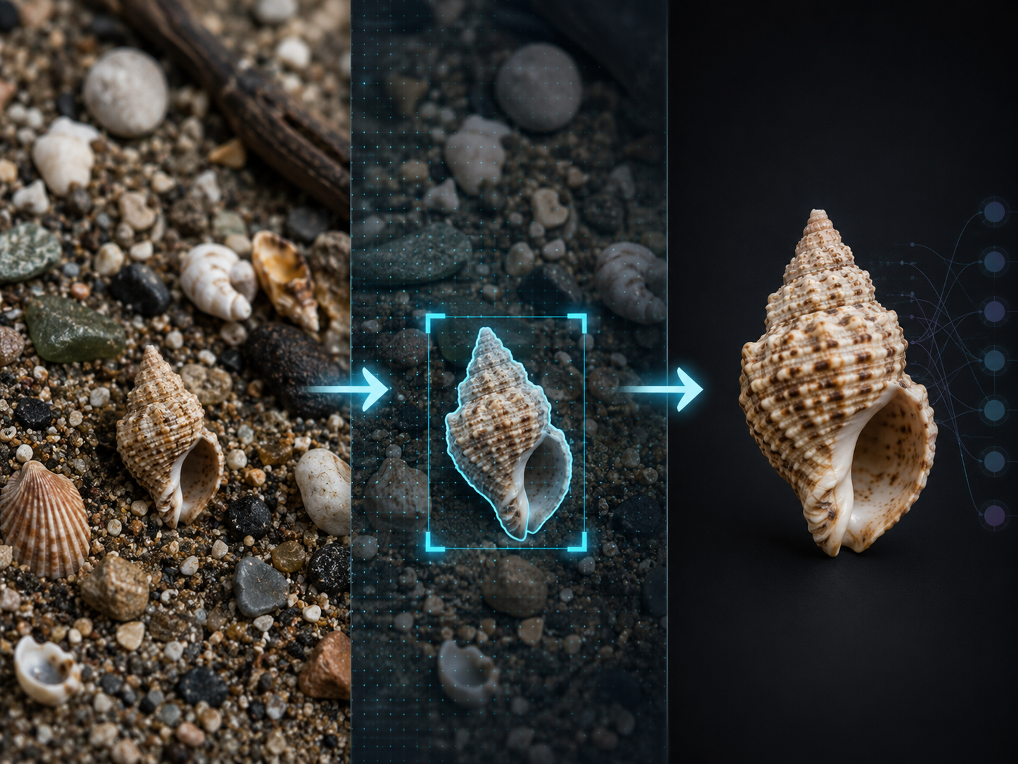
Hierarchical CNN to identify Mollusca
Published on: 12 January 2025
Abstract
Deep learning, particularly Convolutional Neural Networks (CNNs), has revolutionized the field of image-based classification. However, most CNN applications rely on flat classification structures, overlooking the nested relationships inherent in many real-world tasks. This study investigates a hierarchical CNN framework for the taxonomic classification of Mollusca species, leveraging the modularity and flexibility of a “Local Classifier per Parent Node” (LCPN) architecture. Each node in the taxonomic hierarchy (e.g., family, genus, species) is assigned a specialized CNN model, enabling individualized hyperparameter tuning and allowing each model to capture the morphological nuances specific to its target group.
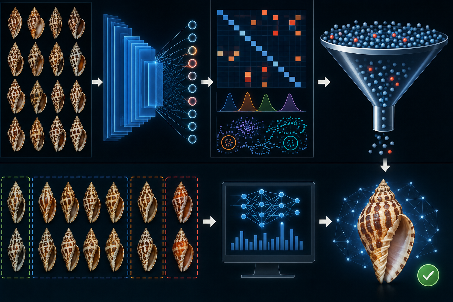
We construct a hierarchy of CNNs, from the phylum level down to individual genera and species, and address dataset imbalances through class weighting, focal loss, data augmentation, and undersampling. Empirical results underscore the effectiveness of our hierarchical architecture, showing improvements in predictive performance and robustness compared to a monolithic, flat classification model. Analyses within the family Cypraeidae reveal that genus-specific morphological features, rather than dataset size or class counts, most strongly impact model accuracy. By reducing classification errors at each taxonomic tier, the hierarchical approach offers finer control and interpretability of classifications — a key advantage for biodiversity monitoring, ecological research, and conchology.
Overall, our findings affirm that a hierarchical CNN framework provides significant gains in accuracy, scalability, and adaptability for complex taxonomic tasks, underscoring its potential for broader applications in biological taxonomy and beyond.
Introduction
In recent years, Convolutional Neural Networks (CNNs) have emerged as a dominant paradigm in machine learning, particularly for tasks
involving image recognition, object detection, and classification. Their architecture, inspired by the human visual system, enables them
to effectively capture spatial hierarchies in data, making them highly effective for extracting features across varying
levels of granularity. While CNNs have demonstrated remarkable success in numerous domains, most applications are designed
to produce flat, single-level predictions, without explicitly leveraging the hierarchical relationships inherent in many
classification tasks.
Hierarchical classification tasks, such as taxonomic classification of species, inherently
involve nested relationships between classes. For example, biological taxonomies organize organisms in a hierarchy of taxonomic
ranks (e.g., class, order, family, and species), while diseases are categorized by systems and subtypes. Exploiting these
hierarchical structures within a classification framework has the potential to improve both the accuracy and interpretability
of machine learning models. Hierarchical CNNs, which either embed hierarchical structures into a single model or use a collection of CNN models
working together hierarchically, represent a promising approach to address this challenge.
The concept of hierarchical CNNs encompasses two primary strategies. The first approach integrates hierarchical relationships directly
into the architecture or loss function of a single CNN, enabling it to model dependencies among different levels of classification.
The second approach involves a collection of CNN models, each specialized to operate at a specific level of the hierarchy, progressively
refining predictions from coarse categories (e.g., order, family) to finer ones (e.g., species). This latter method closely mirrors the
hierarchical decision-making processes, where general categories are identified first, followed by finer distinctions.
Hierarchical CNNs have shown potential in domains like taxonomy, where large datasets often contain imbalances across levels of the hierarchy.
This paper explores the application of hierarchical CNNs in Mollusca. We discuss the advantages of leveraging hierarchical structures and
analyze existing methodologies.
Hierarchical Classification in Biological Taxonomy Using CNNs on Images
CNNs are a widely used to detect and classify organisms. It is common to use a traditional “flat” classification, whereby CNN models do not explicitly consider evolutionary relationships between taxa [1]. However, hierarchical classification has been applied in deep learning to manage large datasets with numerous classes effectively. For the Mollusca dataset presented here, which includes over 100,000 species [11], a hierarchical classification approach is particularly well-suited. Hierarchical classification was attempted for many organism such as arthropods [3]. Tresson et al. (2021)[3] used a two-step approach, first classifying arthropods in five super-classes and then using another model to classify cropped images at the species level. Ong SQ & Hamid SA. [4] have shown the each taxonomic level has its optimal algorithm. Moreover each taxon gave a different performance. They demonstrated that a single deep learning architecture was not robust enough to classify different taxonomic levels of specimens. Another approach was used by Wu et al. [6]. They used a hierarchical cross-entropy (HXE) loss function to organize a “flat” network of leaves in a tree. However, results varied widely among different datasets. Gupta et al. [4] used an hierarchical classification together with YOLOv3 object detection in fish. The same approach is used by Iwano et al [14]. They developed a hierarchical framework that combines YOLOv7 and EfficientNetV2, demonstrating its efficacy in plant disease diagnosis and hierarchical classification. While hierarchical classification has already been developed for species classification, it has to our knowledge not been carried out for Mollusca.Approaches to use CNN for Hierarchical Classification
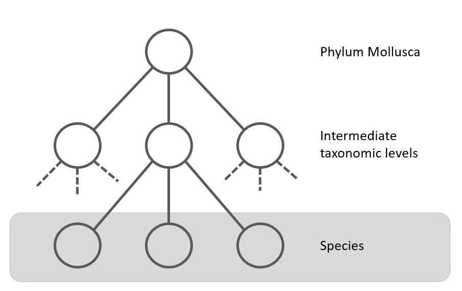
Figure 1: "Flat" classification approach using a multi-class classifier to predict the leaf nodes (Species). The grey area represents the classifier.
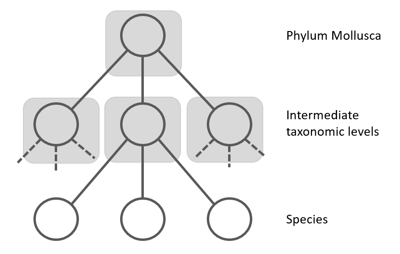
Figure 2: The Local Classifier per Parent Node uses a multi-class classifier to predict the nodes at the next level. The grey squares represent the classifiers.
Another approach is the "Local Classifiers per Parent Node", where separate CNN models for each node in the taxonomic tree is trained. Each classifier is responsible for discriminating between the child nodes of its parent node [13]. It is also known as the top-down approach (see figure 2). In this top-down approach, for each new example in the test set, the system first predicts its first-level (coarse-grained) class, then it uses that predicted class to narrow the choices of classes to be predicted at the second level (the only valid candidate second-level classes are the children of the class predicted at the first level), and so on, recursively, until the most specific (fine-grained) prediction is made. A disadvantage of the top-down class-prediction approach is that an error at one level will be propagated downwards the hierarchy, unless some procedure for avoiding this problem is used (see next chapter). For example, one CNN at the class level to differentiate gastropods from bivalves, then another CNN for gastropods to distinguish orders, and so on
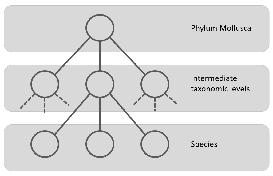
Figure 3: Local Classifier per Level classification approach using a multi-class classifier to classify the nodes at a level. The grey area represents the classifier.
A compromise between the previous two is the Local Classifiers per Level. In this approach one CNN per taxonomic level (one for class, one for order, one for family, etc.) is trained. This means that depending on the higher levels, there are less classes, so the model is trained in the coarse-grained features, while the classifier on the lowest level will be trained on many more classes on the fine-grained features. Figure 3 gives a schematic presentation of this approach. One possible way of classifying test examples using classifiers trained by this approach is when a new test example is presented to the classifier, to get the output of all classifiers (one classifier per level) and use this information as the final classification. This approach was used by S. Kiel on fossil bivalves [20] (a subset of the Mollusca). This research focused on training CNNs at different taxonomic levels (family, order, and subclass) and combining their predictions to address the issue of convergent evolution, where unrelated species develop similar features. The study found that incorporating predictions from higher taxonomic levels improved the accuracy of family-level clustering, particularly for families not included in the training data. This finding supports the concept of hierarchical CNNs being able to leverage broader morphological knowledge to refine fine-grained distinctions. The major drawback of this class-prediction approach is being prone to class-membership inconsistency.
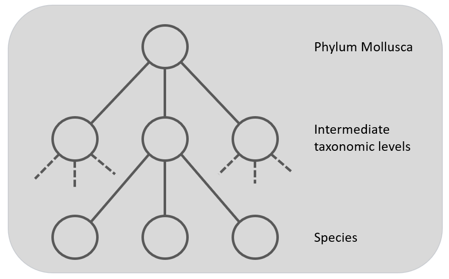
Figure 4: The Global multi-class classifier to predict the nodes at the leaf level but using hierarchy information. The grey squares represent the classifiers.
At last, there is the approach to take the hierarchy into account in a global classifier. This gives a single , but complex, classification model built from the training set. For example, the CNN's loss function could incorporate the hierarchical structure. This approach penalize errors more heavily that are further away in the taxonomic tree [12]. Only one CNN is used to train the complete dataset, so this corresponds with the approach described in figure 1, but with the advantage of having the hierarchy included in the model.
Rationale for using a local classifier per node approach
In this article the "Local Classifier per Parent Node (LCPN) approach [9] was selected. In LCPN a multi-class classifier is trained for each parent node to distinguish between its child nodes. For example, a classifier at the family level would be trained to classify all species within that family. Using a model for each node provides much more flexibility during training of the model. The hyperparameters were optimized for each node.Ong SQ & Hamid SA. [5] have demonstrated that using another model for each taxonomic level gives better results. The hyperparameters were different for each model, which depends on the size of the image dataset, the quality of the images and most important, the morphological features of each taxon (order, family, genus). Some genera have species that are easily to recognize, while other genera have species that are very difficult to identify. Therefore, having specializing classifiers for each node, LCPN can potentially improve overall classification accuracy . Each classifier focuses on a specific subset of the data and learns the distinct characteristics of that taxonomic group. This can be particularly beneficial when dealing with diverse and complex datasets, as is often the case in biological taxonomy.
LCPN has the potential to handle imbalanced datasets at different levels of the hierarchy. In biological taxonomy, certain taxa may have significantly fewer representatives than others. By training separate classifiers for each node, LCPN can address this imbalance by focusing on the specific characteristics of each group, even if some groups have limited data.
This allows working in an interative manner; adding more nodes over time. It enables also more experimentation because the time and IT resources to train a model for a new node, especially the leaves in the tree. At last, because the Mollusca taxonomy changes regularly, only a few nodes need new training.
At last, this approach is cost effective because it requires much less IT infrastructure when compared to training on the complete dataset of images.
A common disadvantage of this approach is the potential for inconsistencies in classification across different levels of the hierarchy . This can occur when a classifier at a lower level assigns an instance to a class that contradicts the classification made by a classifier at a higher level. For example, when classifying mammals, if a classifier at the order level assigns a specimen to the order Primates, but a classifier at the family level assigns it to the family Felidae (cats), this creates an inconsistency. But because an top-down approach is followed during inference time, no inconsistencies will occur. This involves starting at the root of the hierarchy and progressing down, using the predictions at each level to guide the selection of the next classifier. Thresholds can be applied to the classifier outputs to ensure that an instance is only assigned to a child node if the parent node's prediction exceeds a certain confidence level [9]
Another challenge is the increased complexity of managing and training a large number of individual classifiers, especially in a complex hierarchy like biological taxonomy . This requires a careful design of the inference process. [10] Using efficient algorithms and data structures can help reduce the computational burden of training and managing multiple classifiers. This could involve optimizing the code for specific IT architectures or using specialized libraries for hierarchical classification.
Methods
Data collection
Data collection was described previously. All taxonomic information was retrieved from MolluscaBase [11] or Worms [19] To have a reliable classification success a minimum of 25 images per species are needed.Training and testing the convolutional neural network
Model selection was described here. For each node in the taxonomy, the hyperparameters were optimized. The following table shows starting values.Default hyperparameters
| Hyperparameter | Initial value |
|---|---|
| Epochs | 50 |
| Learning rate | 0.0005 |
| Early stopping | Yes |
| Batch Size | 64 |
| Dropout top layer | 0.20 |
| Optimizer | Adam |
| Early stopping | Yes |
Model evaluation
The output layer (softmax) of the CNN consisted of a vector with a confidence value for each class (i.e., taxon) included in the model. The class with the highest value is the predicted class for an image. We assessed if the image was predicted correctly, if the ground truth name class is the same. The python module sklearn.metrics was used to calculate all common metrics: recall, precision, F1 score and accuracy.Results
Criteria to create the tree structure
The taxonomic tree for Mollusca can have many levels, for example the tree for Callista chione (Linneaeus, 1758), a bivalve from the North Atlantic Ocen and Mediterranean Sea, is given below [11]. There are 12 taxonomic levels in this example between Mollusca and the species, Callista choine in this example.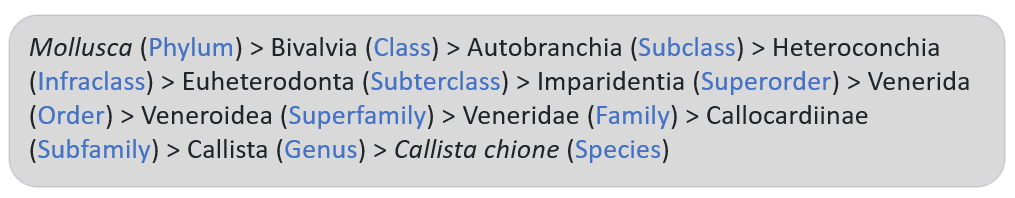
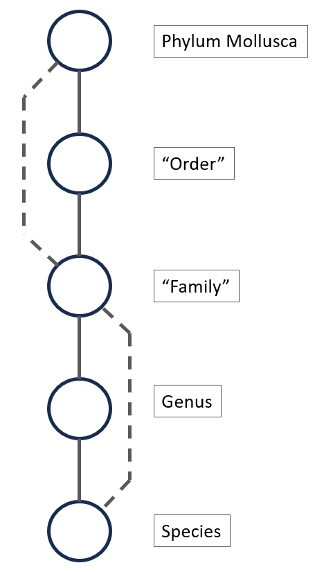
Figure 6.
If not enough species are available in a particular genus (for example, only one or two species with enough images), it might be more efficient to create a model that classifies the species starting from the family. This is shown in figure 6 with the second dotted line. This hierarchical approach ensures an efficient and targeted classification process, with each CNN model specializing in specific levels of the taxonomy.
The root model: Mollusca
The classes selected for the first taxonomic level, the Mollusca (Phylum) parent node are listed in the next table. It has 22 classes, which classify molluscs at the "order" level (see figure 6). The taxonomic level is given in table I, and can be subterclass, infraclass, order, superfamily or family. When the class has the taxonomic level family, we consider this first level to be skipped (see figure 6). The last column shows the number of images available for the class. There is a large imbalance in the dataset.Table I: Classes of the Mollusca model
| Name Taxon | Taxonomic level | # Images |
|---|---|---|
| Archiheterodonta | Subterclass | 1473 |
| Arcida | Order | 5567 |
| Caenogastropoda incertae sedis | Order | 14023 |
| Chitonida | Order | 800 |
| Cycloneritida | Order | 8072 |
| Dentaliidae | Family | 473 |
| Euheterodonta | Subterclass | 16658 |
| Euthyneura | Infraclass | 4637 |
| Lepetellida | Order | 14463 |
| Lepidopleurida | Order | 434 |
| Limida | Order | 1408 |
| Littorinimorpha | Order | 131468 |
| Lottioidea | Superfamily | 1884 |
| Mytilida | Order | 4542 |
| Neogastropoda | Order | 170973 |
| Nuculanoidea | Superfamily | 540 |
| Nuculoidea | Superfamily | 1067 |
| Patelloidea | Superfamily | 5322 |
| Pectinida | Order | 11878 |
| Pleurotomariida | Order | 3182 |
| Seguenziida | Order | 638 |
| Trochida | Order | 20693 |
Table II: Performance of all classes of the Mollusca model
| Name Taxon | Recall | Precision | F1 |
|---|---|---|---|
| Archiheterodonta | 1.000 | 1.000 | 1.000 |
| Arcida | 0.386 | 0.809 | 0.523 |
| Caenogastropoda incertae sedis | 0.982 | 0.823 | 0.896 |
| Chitonida | 1.000 | 0.428 | 0.600 |
| Cycloneritida | 0.958 | 0.884 | 0.920 |
| Dentaliidae | 1.000 | 0.500 | 0.666 |
| Euheterodonta | 0.947 | 0.831 | 0.885 |
| Euthyneura | 1.000 | 0.900 | 0.947 |
| Lepetellida | 0.951 | 0.975 | 0.963 |
| Lepidopleurida | 1.000 | 1.000 | 1.000 |
| Limida | 1.000 | 0.833 | 0.909 |
| Littorinimorpha | 0.975 | 0.987 | 0.981 |
| Lottioidea | 1.000 | 0.500 | 0.666 |
| Mytilida | 0.944 | 0.894 | 0.918 |
| Neogastropoda | 0.973 | 0.989 | 0.981 |
| Nuculanoidea | 1.000 | 0.166 | 0.285 |
| Patelloidea | 0.888 | 0.841 | 0.864 |
| Pectinida | 1.000 | 1.000 | 1.000 |
| Pleurotomariida | 1.000 | 0.833 | 0.909 |
| Seguenziida | 1.000 | 0.800 | 0.888 |
| Trochida | 0.958 | 0.985 | 0.971 |
| Class weights were used, but no other adjustments were made to improve the imbalance. The 3 top layers were unfrozen and a regularization value of 0.0001 was used. All other parameters had default values. The dataset has 424406 images. | |||
Table III: Focal loss, augmentation and undersampling
| # images | Accuracy | Loss | Dentaliidae | Nuculanoidae | Littorinimorpha | Neogastropda | |||||||
|---|---|---|---|---|---|---|---|---|---|---|---|---|---|
| Total | Max. per class | Training | Validation | Training | Validation | F1 Score | # images | F1 Score | # images | F1 Score | # images | F1 Score | # images |
| 12235 | 1000 | 0.986 | 0.938 | 0.010 | 0.033 | 0.928 | 473 | 0.914 | 540 | 0.849 | 1000 | 0.870 | 1000 |
| 26526 | 2500 | 0.989 | 0.959 | 0.009 | 0.025 | 0.914 | 473 | 0.980 | 540 | 0.943 | 2500 | 0.897 | 2500 |
| 44485 | 5000 | 0.983 | 0.964 | 0.012 | 0.022 | 1.000 | 473 | 0.923 | 540 | 0.952 | 5000 | 0.948 | 5000 |
| 68895 | 10000 | 0.985 | 0.971 | 0.012 | 0.018 | 1.000 | 473 | 0.870 | 540 | 0.967 | 10000 | 0.930 | 10000 |
| 103489 | 25000 | 0.980 | 0.971 | 0.012 | 0.019 | 1.000 | 473 | 0.875 | 540 | 0.961 | 25000 | 0.963 | 25000 |
| No undersampling | 0.960 | 0.964 | 0.030 | 0.033 | 0.666 | 473 | 1.000 | 540 | 0.981 | 131468 | 0.981 | 170973 | |
All tests with augmentation of the minority classes (rotate, change brightness and contrast and zoom-out) gave no better results (not shown).
We have further fine-tuned the model and made more top layers trainable. This increases the overall performance, where 10 trainable layers is optimal.
Table IV: Fine-tuning
| # images | Accuracy | Loss | Dentaliidae | Nuculanoidae | Littorinimorpha | Neogastropda | |||||||
|---|---|---|---|---|---|---|---|---|---|---|---|---|---|
| Total | Max. per class | Training | Validation | Training | Validation | F1 Score | # images | F1 Score | # images | F1 Score | # images | F1 Score | # images |
| 44485 | 5000 | 0.991 | 0.970 | 0.008 | 0.019 | 1.000 | 473 | 0.952 | 540 | 0.984 | 3000 | 0.937 | 3000 |
| 103489 | 25000 | 0.989 | 0.976 | 0.013 | 0.016 | 1.000 | 473 | 1.000 | 540 | 0.977 | 15000 | 0.970 | 15000 |
| 133389 | 50000 | 0.982 | 0.975 | 0.023 | 0.018 | 0.666 | 473 | 1.000 | 540 | 0.982 | 30000 | 0.979 | 30000 |
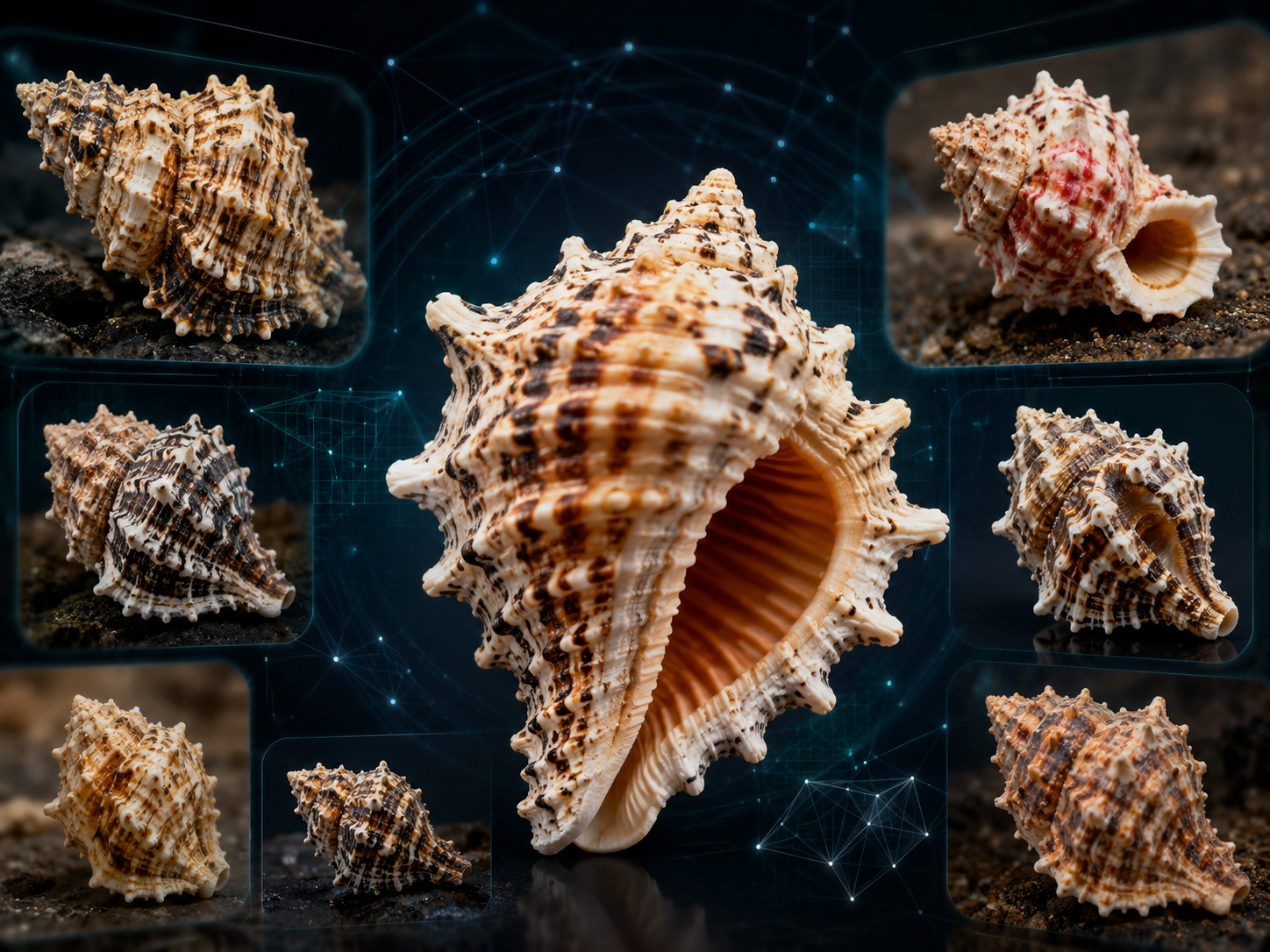
Analyzing the models on genus taxonimic level of the Cypraeidae family
The species of the family Cypraeidae have a similar form, with a wide variation in the pattern and colours. For 18 genera we created models. We have compared these models to see if the hyperparameters correlate with the size of the dataset or the number of classes (species) in the dataset. Table V shows the result of all genera with the same (initial) hyperparameters and the final optimized, fine-tuned models.Table IV: Fine-tuning
| Model with same (initial) hyperparameters | Fine-tuned Model with optimized hyperparameters | |||||||||||||
|---|---|---|---|---|---|---|---|---|---|---|---|---|---|---|
| Genus | # images | # species | Train. Acc. | Val. Acc. | Train. Loss | Val. Loss | Learning rate | Top layer dropout | Un-freezed top layers | Regulari-zation | Train. Acc. | Val. Acc. | Train. Loss | Val. Loss |
| Austrasiatica | 1396 | 3 | 0.942 | 0.943 | 0.248 | 0.203 | 0.0005 | 0.2 | - | - | 0.942 | 0.943 | 0.248 | 0.203 |
| Bistolida | 4440 | 11 | 0.837 | 0.837 | 0.266 | 0.075 | 0.001 | 0.2 | 20 | 0.01 | 0.965 | 0.919 | 0.087 | 0.085 |
| Cypraeovula | 3830 | 14 | 0.885 | 0.876 | 0.867 | 0.885 | 0.0005 | 0.2 | 3 | 0.0001 | 0.956 | 0.914 | 0.266 | 0.289 |
| Eclogavena | 2110 | 5 | 0.892 | 0.879 | 0.485 | 0.376 | 0.00025 | 0.2 | 3 | - | 0.959 | 0.950 | 0.182 | 0.189 |
| Erronea | 9338 | 16 | 0.860 | 0.892 | 1.122 | 0.362 | 0.0005 | 0.2 | 3 | 0.0001 | 0.953 | 0.935 | 0.324 | 0.211 |
| Leporicypraea | 2394 | 4 | 0.913 | 0.914 | 0.546 | 0.244 | 0.0005 | 0.2 | 3 | 0.0001 | 0.968 | 0.960 | 0.155 | 0.126 |
| Lyncina | 9210 | 11 | 0.912 | 0.934 | 1.279 | 0.226 | 0.0005 | 0.2 | 3 | 0.0001 | 0.978 | 0.964 | 0.291 | 0.123 |
| Mauritia | 8299 | 8 | 0.815 | 0.853 | 0.125 | 0.051 | 0.0005 | 0.2 | 3 | 0.0001 | 0.953 | 0.919 | 0.024 | 0.031 |
| Melicerona | 623 | 2 | 0.938 | 0.863 | 0.230 | 0.293 | 0.00025 | 0.25 | 3 | 0.0001 | 0.96 | 0.903 | 0.157 | 0.241 |
| Naria | 23518 | 24 | 0.879 | 0.925 | 0.924 | 0.296 | 0.001 | 0.1 | 3 | 0.0001 | 0.987 | 0.965 | 0.018 | 0.026 |
| Notocypraea | 2230 | 5 | 0.825 | 0.796 | 0.659 | 0.559 | 0.001 | 0.2 | 3 | 0.001 | 0.959 | 0.888 | 0.167 | 0.408 |
| Palmadusta | 7058 | 13 | 0.947 | 0.945 | 0.278 | 0.175 | 0.0005 | 0.2 | - | - | 0.947 | 0.945 | 0.278 | 0.175 |
| Pseudozonaria | 1753 | 4 | 0.962 | 0.980 | 0.152 | 0.089 | 0.0005 | 0.2 | - | - | 0.962 | 0.980 | 0.152 | 0.089 |
| Purpuradusta | 2575 | 8 | 0.870 | 0.849 | 1.233 | 0.533 | 0.0005 | 0.2 | 3 | 0.0001 | 0.932 | 0.882 | 0.663 | 0.650 |
| Pustularia | 4332 | 10 | 0.837 | 0.848 | 0.854 | 0.471 | 0.0005 | 0.2 | 20 | 0.01 | 0.967 | 0.916 | 0.050 | 0.060 |
| Talparia | 1075 | 2 | 0.949 | 0.977 | 0.222 | 0.086 | 0.0005 | 0.2 | - | - | 0.949 | 0.977 | 0.222 | 0.086 |
| Umbilia | 2898 | 7 | 0.846 | 0.889 | 0.947 | 0.341 | 0.0005 | 0.2 | 3 | - | 0.941 | 0.941 | 0.408 | 0.213 |
| Zoila | 7036 | 27 | 0.855 | 0.848 | 1.264 | 0.502 | 0.0005 | 0.2 | 3 | 0.0001 | 0.977 | 0.916 | 0.231 | 0.299 |
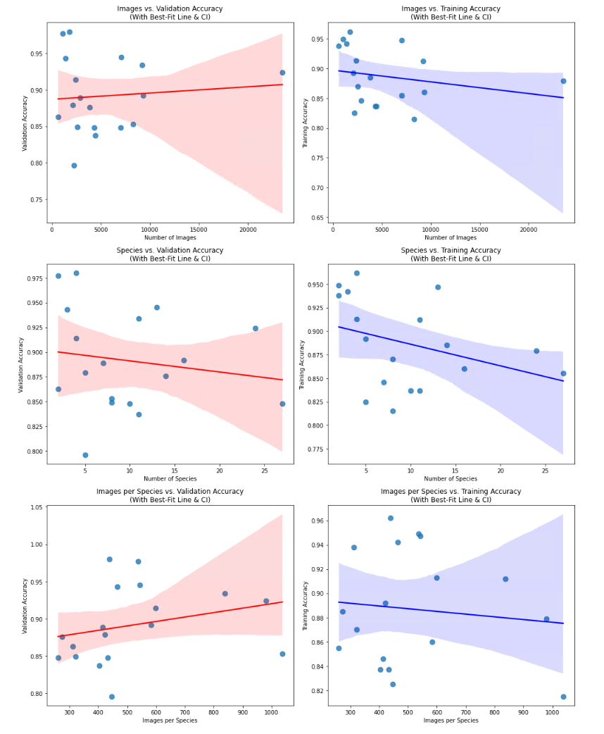
Using the same parameters for the first training (see default parameters), the results vary widely between a training accuracy of 0.815 for the Mauritia model until 0.962 for the Pseudozonaria model. Optimizing the hyperparameters and further fine-tuning gave always better results, all models having at least a validation accuracy of 0.9. When plotting the amount of images in the dataset, or the number of species (classes) in the dataset against the accuracy, no correlation was found. The size of the dataset is not able to explain the variation in accuracy among the models.
Conclusion
This study has successfully demonstrated the power of hierarchical convolutional neural networks (CNNs) as a robust tool for the identification of Mollusca species. Our results provide compelling evidence for the efficacy of hierarchical classification strategies, which can be implemented through diverse architectures. These range from a single, end-to-end CNN capable of refining predictions from coarse taxonomic levels (e.g., class) down to fine-grained distinctions (e.g., species), to an ensemble of interconnected CNNs, where each model is specialized for a specific node within the taxonomic hierarchy. In this work, we elected to pursue the latter approach, constructing a hierarchical network of independent CNNs. As detailed in previous sections, this architectural decision was driven by the inherent advantages it offers in terms of modularity, optimization, and feature specificity. The strong performance of our model validates this choice and underscores the potential of hierarchical CNNs for accurate and efficient Mollusca classification.
The observed variations in performance across different taxonomic groups, particularly within the family Cypraeidae, offer critical insights into the benefits of our chosen architecture. By utilizing a dedicated model for each node within the hierarchy, we are empowered to fine-tune hyperparameters at each level of classification. This granular level of optimization ensures that each model is ideally suited to the specific challenges posed by its target taxonomic group. Consequently, this strategy leads to demonstrably superior outcomes compared to a single, "flat" model attempting to classify all Mollusca species simultaneously. In such a monolithic approach, optimal hyperparameters for one group might prove detrimental to another, hindering overall accuracy.
Furthermore, the adoption of a hierarchical network of specialized models allows each CNN to focus on learning the distinct morphological characteristics relevant to its assigned genus. Our findings suggest that the presence of these genus-specific features is a more significant determinant of model performance than either the sheer size of the dataset or the total number of classes within a given node. This implies that even within a complex and diverse group like Mollusca, a well-structured hierarchy can leverage subtle, genus-level morphological differences to achieve accurate identification.
The success of our hierarchical CNN approach has significant implications for the field of conchology and biodiversity research. It provides a framework for developing automated, accurate, and efficient tools for species identification, which can be invaluable for tasks such as biodiversity monitoring, ecological surveys, conservation efforts and shell collection. Investigating the interpretability of the learned features within each model could provide further insights into the specific morphological characteristics that distinguish different Mollusca genera and species.
References
- [1] Hansen OL, et al. Species-level image classification with convolutional neural network enables insect identification from habitus images. Ecology and Evolution 10(2), (2020).
- [2] Kittichai V et al. Deep learning approaches for challenging species and gender identification of mosquito vectors. Scientific Reports 11(1), (2021).
- [3] Tresson P et al. Hierarchical Classification of Very Small Objects: Application to the Detection of Arthropod Species. IEEE Access 9 (2021) .
- [4] Gupta DA et al. Hierarchical Object Detection applied to Fish Species. Nordic Machine Intelligence 2(1):1–15 (2022).
- [5] Ong SQ & Hamid SA. Next generation insect taxonomic classification by comparing different deep learning algorithms. PloS one 17(12), (2022).
- [6] Wu C et al. A hierarchical loss and its problems when classifying non-hierarchically. PLoS ONE 14(12):1– 19, (2019).
- [7] Gao D. Deep Hierarchical Classification for Category Prediction in E-commerce System. In: Proceedings of the 3rd Workshop on e-Commerce and NLP. Association for Computational Linguistics p. 64–8, (2020).
- [8] Milan Krendzelak & Frantisek Jakab Hierarchical text classification using CNNs with local approaches Computing and Informatics, Vol. 39, 907–924, (2020).
- [9] Carlos Silla & Alex Freitas A survey of hierarchical classification across different application domains Data Mining and Knowledge Discovery 22(1):31-72, (2011).
- [10] Pâmela M Rezende et al. Evaluating hierarchical machine learning approaches to classify biological databases Brief Bioinform. 21;23(4), (2022).
- [11] MolluscaBase https://www.molluscabase.org/.
- [12] D. Wu et al. Deep learning with taxonomic loss for plant identification Comput. Intell. Neurosci., vol. 2019, pp. 1–8, (2019).
- [13] J. G. Colonna et al. A comparison of hierarchical multi-output recognition approaches for anuran classification Mach. Learn., vol. 107, no. 11, pp. 1651–1671, (2018).
- [14] Iwano, K. et al Hierarchical object detection and recognition framework for practical plant disease diagnosis. https://arxiv.org/abs/2407.17906, (2024).
- [15] Dablain, D. et al. Understanding CNN fragility when learning with imbalanced data. Mach Learn 113, 4785–4810 (2024).
- [16] Pasupa, K. et al Convolutional neural networks based focal loss for class imbalance problem: a case study of canine red blood cells morphology classification Journal of Ambient Intelligence and Humanized Computing 14(11), 15259-15275, (2020).
- [17] Dablain, D. et al Efficient Augmentation for Imbalanced Deep Learning arXiv:2207.06080, (2022).
- [18]Joloudari, J.H. et al Effective Class-Imbalance learning based on SMOTE and Convolutional Neural Networks arXiv:2209.00653, (2022).
- [19] WoRMS - World Register of Marine Species https://www.marinespecies.org/.
- [20]S. Kiel Assessing bivalve phylogeny using Deep Learning and Computer Vision approaches https://doi.org/10.1101/2021.04.08.438943 (2021).