Leakage-Aware and Audit-Governed CNN Classification of Clathurellidae (Conoidea; Gastropoda) Shell Images
Published on: July, 2026

Abstract
Clathurellidae is a morphologically recognizable but internally heterogeneous family of predatory marine gastropods in which species identification from shell images requires fine-grained discrimination among visually similar taxa. This study evaluated a direct Family→Species classifier for 26 Clathurellidae species distributed across eight genera and examined how leakage-aware partitioning and conservative training-data auditing affected the resulting performance estimates. The initial dataset contained 2,295 standardized shell images. Images associated with the same specimen, listing or known duplicate group were retained within a single partition, producing 1,837 training images and 458 held-out validation images. Before production training, the training partition was audited using frozen DINOv3 embeddings, group-aware out-of-fold logistic regression, nearest-neighbour evidence, Cleanlab label-quality estimates and technical review. No image satisfied the complete statistical-quarantine rule, whereas nine technically unusable images were excluded, yielding a final training set of 1,828 images. The production classifier used an ImageNet-pretrained EfficientNetV2B2 model with partial fine-tuning and focal loss. Accuracy decreased from 87.800% under the original partition to 84.716% under the leakage-aware evaluation, while macro F1 decreased from 88.254% to 83.280%. Excluding the nine technical failures did not change overall accuracy: both the pre-audit and audit-filtered models correctly classified 388 of 458 validation images. The final audit-filtered model achieved a weighted F1-score of 84.077% and a macro F1-score of 83.393%. Species-level F1-scores ranged from 0.545 to 1.000; 17 of the 26 species reached at least 0.80, while six were classified perfectly within their validation cohorts. Most residual errors were intrageneric and were concentrated within Lienardia and Etrema. Equalizing species support reduced accuracy to 82.290%, confirming that reliability was not uniform across the label space. These results show that standardized shell images support effective identification of many included Clathurellidae species, but also demonstrate the importance of leakage-aware evaluation, conservative data curation and species-level reporting. The resulting classifier should be interpreted as a controlled benchmark for the 26 included species rather than as a complete identification system for Clathurellidae.
Introduction
Clathurellidae H. Adams & A. Adams, 1858 is a family of predatory marine gastropods within the superfamily Conoidea. Its present circumscription is the result of a substantial reorganisation of conoidean systematics. For much of the twentieth century, many clathurellid and related lineages were included within the broadly defined and morphologically heterogeneous “Turridae”. Early molecular analyses demonstrated that this traditional assemblage was not monophyletic and that shell- and radula-based classifications did not consistently recover evolutionary relationships [1]. Expanded molecular sampling subsequently resolved the former “turrids” into multiple family-level lineages and provided the phylogenetic basis for recognizing Clathurellidae as a separate family [2], [3]. This family-level treatment was retained in the later revised classification and nomenclator of gastropod families [12].
Later mitogenomic and phylogenomic studies strengthened support for Clathurellidae as a distinct conoidean lineage. Mitochondrial-genome analyses placed it among a group of closely related toxoglossate families that also includes Mangeliidae, Mitromorphidae, Raphitomidae, Borsoniidae and Conidae [9]. Exon-capture phylogenomics based on hundreds of nuclear loci recovered strong support for Clathurellidae while also showing that the precise relationships among several neighbouring conoidean families remain sensitive to taxon sampling and the molecular data used [8]. Focused molecular work on Raphitomidae and allied groups has likewise shown that some genera historically placed near or within Clathurellidae require reassignment when molecular and anatomical evidence are considered together [11]. The family-level concept is therefore substantially more stable than many of its historical generic associations.
Clathurellidae nevertheless retains a recognizable conchological identity. The shells are generally small to medium-sized and commonly fusiform, biconic or narrowly turriform, with an elevated spire and prominent axial and spiral sculpture. Intersections between axial ribs and spiral cords frequently produce a cancellate or reticulate surface. The family diagnosis also includes a deep anal sinus positioned on or against the sutural ramp, absence of true columellar pleats, consistent loss of the operculum, and hollow hypodermic marginal radular teeth associated with the conoidean predatory apparatus [3]. These characters distinguish the family as a whole, but their expression varies considerably among genera and species.
Shell morphology is therefore both informative and incomplete for identification. Similar combinations of axial ribs, spiral cords, apertural denticles and shell proportions can occur in several clathurellid lineages, while viewing angle, preservation, erosion, colour variation and growth stage can alter the characters visible in an image. Conversely, characters not represented consistently in ordinary shell photographs—including the protoconch, radula, soft-part anatomy and developmental traits—may contribute substantially to taxonomic diagnosis. In Lienardia, for example, correlations among radular morphology, protoconch colour and adult shell colour pattern supported the continued separation of Lienardia from Clathurella [10]. This illustrates why visual similarity in the adult shell cannot always be treated as equivalent to taxonomic or phylogenetic identity.
These properties make Clathurellidae a relevant test case for image-based species classification. A convolutional neural network trained on standardized shell images does not test phylogenetic relationships and cannot evaluate anatomical or molecular characters that are absent from the image. It does, however, measure how consistently the current species labels can be recovered from the visible shell representation. Strong and uniform performance indicates that the available images contain a reproducible visual signal for a species. Weak or uneven performance may arise from limited sample support, image-quality variation, incomplete diagnostic views, intraspecific variation, interspecific shell similarity or heterogeneous taxonomic labels. Classification performance should therefore be interpreted as a benchmark of visual diagnosability rather than as a taxonomic revision.
The reliability of such a benchmark also depends on the construction of the image dataset. Online shell collections may contain several photographs of the same specimen, repeated listings, transformed copies of the same source image, identification labels instead of specimens, technically unusable images and potentially inconsistent species assignments. When related images are distributed between training and validation partitions, the resulting evaluation does not represent fully independent specimen-level recognition. Conversely, removing difficult images solely because a preliminary classifier disagrees with their labels can simplify the task artificially and discard genuine morphological variation. Dataset partitioning and auditing must therefore separate demonstrable technical defects from statistical disagreement and taxonomic ambiguity.
The present study evaluates a direct Family→Species classifier for 26 Clathurellidae species distributed across eight genera. An EfficientNetV2B2 model was first evaluated through a series of fine-tuning configurations on the original dataset partition. The selected configuration was then applied to a leakage-aware partition in which images belonging to the same specimen, listing or duplicate group were kept together. Before final production training, the training partition was examined using frozen DINOv3 embeddings, group-aware out-of-fold classification, nearest-neighbour evidence, Cleanlab label-quality estimates and technical review. Statistical disagreement was retained unless it satisfied a conservative conjunctive exclusion rule, whereas directly unusable training images could be assigned to technical quarantine.
The study addresses four related questions. First, how much did the aggregate evaluation change when the original partition was replaced by a leakage-aware partition? Second, did exclusion of the audit-identified technical failures materially change performance on the unchanged held-out validation cohort? Third, which species and species pairs remained visually difficult after leakage control and auditing? Finally, how did performance differ between the natural validation distribution and an evaluation in which every species contributed equal record support? Together, these analyses assess both the operational performance of the Clathurellidae classifier and the extent to which current species labels are recoverable from standardized shell imagery.
Methods
Data acquisition and taxonomic normalization
The image corpus was assembled through the existing IdentifyShell data-collection workflow from multiple publicly accessible and specialist sources. These included biodiversity repositories, institutional and university image collections, specialist malacological websites, commercial shell collections and selected online marketplace listings. Available source, listing and specimen information was retained when possible so that repeated listings, multiple views of the same specimen and known duplicate images could be recognized during dataset preparation.
Taxonomic names and family assignments were checked against WoRMS and MolluscaBase [4] during dataset construction. Accepted species names were used as model classes. Records published under recognized synonyms were assigned to the corresponding accepted name, whereas records that could not be resolved to an accepted species-level identification were not eligible for inclusion. This standardisation was intended to provide a consistent operational label set and should not be interpreted as an independent taxonomic revision of Clathurellidae.
Taxonomic scope and species inclusion criteria
Species were eligible for the family-to-species model when at least 25 transformed images were available after taxonomic and image-level preprocessing. The retained classes represented eight genera: Clathurella with two species, Corinnaeturris with one, Etrema with six, Lienardia with thirteen, Nannodiella with one, Paraclathurella with one, Pseudoetrema with one and Strombinoturris with one.
A genus represented by one included species was not assumed to be biologically monospecific. It indicates only that one species from that genus met the identification, image-availability and preprocessing requirements of the present dataset. Species and genera falling below the eligibility threshold remained outside the model label space.
The resulting taxonomic coverage reflects the availability of usable and sufficiently identified online shell images rather than balanced or exhaustive sampling of Clathurellidae diversity. The complete species inventory and the class-specific counts at each dataset stage are provided in Supplementary Table S1.
Image preprocessing and transformed-image construction
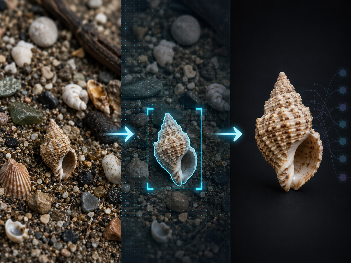
Before partitioning, eligible source photographs were converted into standardized shell-centred image records using the established IdentifyShell preprocessing workflow. The shell was detected and isolated from the source photograph, and non-shell elements such as identification labels, rulers, hands and surrounding scene content were removed where technically feasible. A uniform black background and square padding were applied where required, and the resulting images were stored at 400 × 400 pixels.
Each stored transformed image was treated as one dataset observation. Different photographs or views of the same underlying specimen could therefore remain as separate image records, but they retained a common specimen, listing or duplicate group when that relationship was known. These relationships were subsequently used by the leakage-aware partitioning procedure.
The reported dataset counts refer to these stored natural image records. On-the-fly augmentation or repeated sampling during model fitting did not create additional unique dataset images.
Dataset composition and leakage-aware partitioning
The Clathurellidae model was developed as a direct family-to-species classifier, following the general training approach previously used for other family-level models. The principal methodological change in the present study concerned the preparation and auditing of the training data before production-model training.
Two earlier investigations motivated this extension of the pipeline. First, the Morum experiments demonstrated that images originating from the same specimen, listing or duplicate group must not be distributed across training and validation partitions, because such overlap can produce optimistic estimates of model performance [5]. Second, the Harpa study showed that out-of-fold predictions, nearest-neighbour evidence and Cleanlab label-quality estimates can be combined to identify a small number of strongly contradicted training labels while retaining ambiguous or taxonomically difficult images [7].
These findings were incorporated into the Clathurellidae workflow as two upstream controls:
- leakage-aware partitioning before any model fitting or dataset audit; and
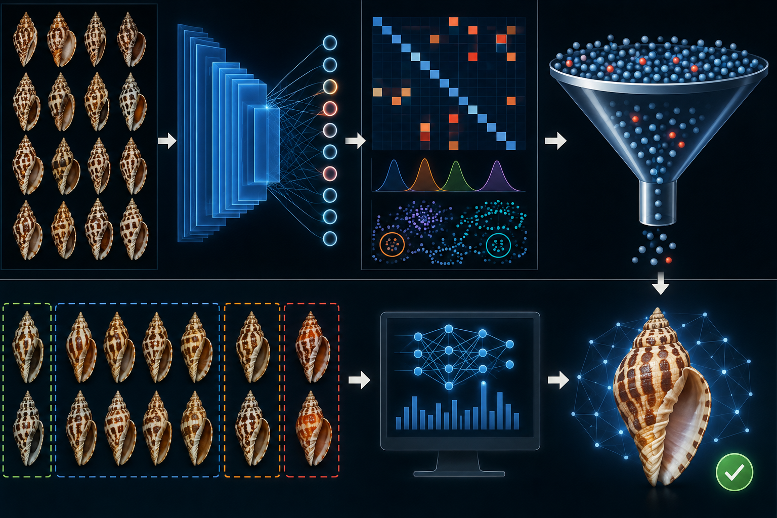
- a reproducible pre-training audit combining frozen DINOv3 embeddings, group-aware out-of-fold classification, nearest-neighbour evidence, Cleanlab analysis and technical-quality review.
The audit used for Clathurellidae differed from the methodology applied in the earlier Harpa experiments. In the present pipeline, frozen DINOv3 representations and lightweight logistic-regression classifiers were used to generate out-of-fold evidence before training the production image-classification model. The audit was therefore designed as a computationally efficient and reusable data-quality stage rather than as an evaluation of the final convolutional neural network itself. Statistical exclusion remained deliberately conservative because the resulting probabilities originated from a linear classifier fitted to frozen embeddings rather than from the subsequently trained production model.
The initial Clathurellidae dataset contained 2,295 transformed images representing 26 species. A leakage-aware partitioning procedure was applied before any feature extraction, auditing or model training [5]. Images associated with the same specimen or known duplicate group were assigned to the same partition.
The resulting dataset comprised:
- 1,837 training images; and
- 458 held-out validation images.
The validation partition was isolated throughout the audit. Its images were embedded so that the representations would be available for later diagnostic analyses, but they were not used for fold construction, classifier fitting, label-quality estimation, nearest-neighbour decisions, decision-threshold selection or quarantine calibration.
Consequently, all statistical and technical decisions affecting the training dataset were based solely on evidence derived from the 1,837-image training partition. The validation set remained unchanged and unavailable to the audit decision process.
Extraction of frozen DINOv3 embeddings
All images were encoded using a frozen DINOv3 ViT-S/16 model pretrained on the LVD-1689M dataset [6]. The encoder was used exclusively as a feature extractor. None of its parameters was updated during the audit.
The selected encoder produced one 384-dimensional representation per image and was sufficiently compact to operate on the available GPU hardware. Its purpose was not to replace the production classifier, but to provide a consistent representation space in which out-of-fold classification, nearest-neighbour analysis and label-quality estimation could be performed.
Images were decoded in RGB format and resized to 400 × 400 pixels, corresponding to the input resolution used for subsequent production-model training. Resizing used bilinear interpolation with antialiasing. Images preserved their aspect ratio.
Pixel values were transformed using channel-specific scales of 0.017124754; 0.017507003; and 0.017429194; and corresponding offsets of: −2.11790393; −2.03571429; and −1.80444444.
The class token from the final transformer output was extracted in 32-bit floating-point precision and normalized to unit Euclidean length. The normalized vectors were subsequently stored in 16-bit floating-point format. Because all vectors had unit length, cosine similarity could be calculated as their dot product.
Feature extraction was performed in batches of eight images. Each embedding-cache entry was indexed using:
- the persistent image identifier;
- the SHA-256 hash of the image content;
- the image-transformation hash;
- the encoder fingerprint; and
- the preprocessing fingerprint.
This design allowed unchanged embeddings to be reused while ensuring that a modification to an image, transformation, encoder or preprocessing configuration produced a new cache entry.
The embedding matrix was stored as a contiguous numerical array together with an explicit mapping between matrix rows and persistent image identifiers. Matrix rows were never interpreted independently of this mapping.
The embedding environment used Keras 3.12.3, KerasHub 0.25.1 and TensorFlow 2.20.0.
Group-aware out-of-fold classification
Out-of-fold probabilities were calculated for the 1,837 training images by fitting multinomial logistic-regression classifiers to the frozen DINOv3 embeddings. The 458 validation images did not participate in this procedure.
The training partition was divided into three folds using stratified, group-aware splitting. Stratification attempted to preserve the relative species distribution across folds, while the grouping constraint ensured that every image belonging to the same specimen or duplicate group remained within a single fold.
A proposed split was accepted only when:
- every species was represented in both the fitting and holdout portions of every fold;
- every training image occurred in exactly one holdout fold; and
- no specimen or duplicate group was divided between the fitting and holdout portions of a fold.
Three independent logistic-regression models were then fitted. Each classifier was trained on two folds and used to predict the third. The three sets of holdout predictions were combined to produce one complete probability vector for every training image.
This procedure ensured that an image was never predicted by a classifier trained on that image or on another image belonging to the same specimen or duplicate group.
The classifiers used:
- multinomial logistic regression;
- L2 regularization;
- a regularization parameter of (C=1.0);
- the limited-memory Broyden–Fletcher–Goldfarb–Shanno solver;
- a maximum of 2,000 iterations; and
- no class weighting.
The class order was fixed before model fitting and verified separately for every fold. A convergence warning, missing class or inconsistent class order caused the audit to fail rather than allowing incomplete predictions to propagate into later stages.
Scikit-learn 1.4.1.post1 was used.
For every training image, the stored out-of-fold evidence included:
- the species assigned in the dataset;
- the species predicted by the out-of-fold classifier;
- the complete 26-class probability vector;
- the probability assigned to the dataset label;
- the largest and second-largest predicted probabilities;
- the difference between these probabilities, defined as the prediction margin;
- Shannon entropy of the probability distribution;
- the fold identifier; and
- the specimen- or duplicate-group identifier.
Nearest-neighbour and Cleanlab evidence
Two complementary analyses were applied independently to the training partition: nearest-neighbour analysis in the DINOv3 embedding space and Cleanlab label-quality estimation.
Cosine distances were calculated between the normalized DINOv3 embeddings. The requested neighbourhood size was (k=20).
Before neighbours were selected, the following images were excluded from the candidate pool:
- the query image itself;
- all images belonging to the same specimen or duplicate group; and
- all images with an identical image-content hash.
These exclusions prevented multiple views or transformed copies of the same underlying specimen from artificially inflating neighbourhood agreement.
When fewer than 20 eligible neighbours were available, the number actually retrieved was recorded as the effective neighbourhood size. However, an effective neighbourhood of fewer than 20 images was considered insufficient to support automatic statistical quarantine.
Neighbour support for a species was defined as the unweighted proportion of selected neighbours carrying that species label. For every image, the analysis recorded:
- neighbour support for the assigned species;
- neighbour support for the out-of-fold predicted species;
- the dominant species in the neighbourhood;
- support for the dominant species;
- the effective neighbourhood size; and
- the identifiers, labels and cosine distances of the individual neighbours.
When two or more species had equal support, the species with the smallest mean neighbour distance was selected as the dominant species.
In parallel, label quality was estimated from the observed training labels and the complete out-of-fold probability matrix using Cleanlab 2.9.0.
Label-quality scores were calculated using the self-confidence method. Potential label issues were detected using noise-rate pruning and ranked by self-confidence.
Before Cleanlab was executed, the pipeline verified:
- the image order;
- the number of observed labels;
- the dimensions of the probability matrix;
- the probability sums;
- the class-to-column mapping;
- the persistent image identifiers; and
- the correspondence between the probability rows and image records.
SHA-256 checksums were used to confirm that the transferred probability matrix and its accompanying row mapping had not changed.
A Cleanlab issue flag did not, by itself, constitute evidence that the dataset label was incorrect and did not automatically cause an image to be excluded.
Integration of audit evidence
The out-of-fold predictions, Cleanlab results, nearest-neighbour measurements and available technical-quality evidence were joined using the persistent image identifier.
Before any decision was made, exact agreement was required for:
- the complete set of training-image identifiers;
- the dataset fingerprint;
- the class mapping;
- the encoder fingerprint;
- the preprocessing fingerprint; and
- the out-of-fold run fingerprint.
The audit failed when these elements were incomplete or inconsistent. This prevented evidence generated from different dataset revisions, preprocessing configurations or model installations from being combined inadvertently.
An image was considered a high-contradiction statistical candidate [7] only when all the following conditions were satisfied:
- predicted species \ne assigned species
- largest OOF probability \ge 0.90
- OOF prediction margin \ge 0.50
- Cleanlab label quality \le 0.10
- Cleanlab issue flag = true
- kNN support for assigned species \le 0.20
- kNN support for predicted species \ge 0.80
- dominant kNN species = OOF-predicted species
- effective neighbourhood size \ge 20
- all associated evidence was valid
In addition, all associated evidence had to be present and valid.
The conditions were intentionally conjunctive: disagreement by one method was insufficient. Statistical quarantine required strong and mutually consistent contradiction from the out-of-fold classifier, Cleanlab analysis and local embedding neighbourhood.
The thresholds were deliberately conservative and remained provisional. In particular, the out-of-fold probabilities were generated by logistic regression over frozen DINOv3 representations rather than by the production image-classification model. They were therefore treated as audit evidence rather than as calibrated production probabilities.
Ambiguous and insufficiently supported images
Images with mixed neighbourhoods were retained and marked as ambiguous rather than quarantined.
Technical quarantine was kept separate from statistical quarantine. Automatic technical exclusion required an explicit failure, such as unsuccessful preprocessing, absence of a detected shell, a shell bounding-box area below 1% of the image, or a mask-to-bounding-box ratio below 0.20 or above 0.95. Softer warnings were retained. When matching automated technical measurements were unavailable, this was recorded but did not itself cause exclusion.
A neighbourhood was classified as mixed when:
- its dominant species was neither the assigned species nor the out-of-fold predicted species; or
- support for its dominant species was below 0.60.
Images were also retained when the available evidence was incomplete, the effective neighbourhood was too small or the contradiction thresholds were not satisfied.
This distinction was important because disagreement may arise from genuine morphological similarity, difficult viewing angles, image degradation, limited class support or unresolved taxonomic boundaries. The purpose of the audit was to remove only exceptionally strong statistical contradictions, not to simplify the dataset by discarding difficult examples.
Quarantine safeguards
Additional limits prevented a large number of images from being removed from the complete dataset or from an individual species.
Statistical quarantine was limited to the smaller of:
- 2% of the complete training partition; or
- 50 images.
The following species-level limits were also applied:
- fewer than 50 training images: no more than 5%, with an absolute maximum of 2 images;
- 50–99 training images: no more than 5%, with an absolute maximum of 5 images;
- 100–499 training images: no more than 7.5%, with an absolute maximum of 15 images; and
- at least 500 training images: no more than 10%, with an absolute maximum of 30 images.
For any individual assigned-species/predicted-species combination, quarantine was further limited to half of the applicable species-level limit, with an absolute maximum of 10 images.
When the number of eligible candidates exceeded one of these limits, candidates were ordered deterministically by:
- increasing Cleanlab label-quality score;
- decreasing out-of-fold probability;
- decreasing prediction margin;
- decreasing neighbour support for the predicted species;
- increasing neighbour support for the assigned species; and
- persistent image identifier.
This ordering prioritized images with the strongest combined contradiction while ensuring that repeated executions produced the same decisions.
Technical-quality quarantine
Technical quarantine was evaluated separately from statistical label contradiction. Statistical evidence was not used to classify an image as technically unusable, and a technical defect was not interpreted as evidence of an incorrect species label.
Automatic technical exclusion required an explicit failure, such as:
- unsuccessful image preprocessing;
- failure to detect a shell;
- a shell bounding-box area below 1% of the complete image;
- a mask-to-bounding-box ratio below 0.20; or
- a mask-to-bounding-box ratio above 0.95.
Less severe quality warnings were retained. When matching automated technical measurements were unavailable, the missing evidence was recorded, but the image was not excluded for that reason alone.
A reviewer could additionally classify an image as technically unusable following visual inspection. Manual technical exclusion was restricted to directly observable problems, including:
- an identification label or other documentation instead of a shell specimen;
- absence of a shell;
- depiction of the wrong object;
- severe corruption or obstruction; or
- another defect that made the image unusable for visual model training.
Manual exclusion was not permitted solely because the reviewer considered the taxonomic identification uncertain. The reason, decision time and reviewer action were recorded. Decisions remained reversible, and changing a decision did not alter or overwrite the original audit evidence.
Construction and verification of the audited dataset
The audit did not modify the original dataset. Instead, a new physical copy was constructed for production-model training.
Statistical and technical decisions were resolved using persistent image identifiers. Images classified as retained, ambiguous, protected or insufficiently supported remained in the training partition. Only images carrying an effective statistical- or technical-quarantine decision were omitted from the audited copy.
The leakage-aware directory structure of the source dataset was preserved. All 458 validation images were copied without modification.
Before the audited dataset was released for training, its inventory was compared with the inventory used during embedding extraction. The construction process failed when it encountered:
- a missing expected image;
- an untracked additional image;
- a duplicate persistent identifier;
- an inconsistent relative path; or
- a mismatch between an image and its recorded content hash.
Every copied image was verified against the SHA-256 hash of its source file. The dataset was made available to the production-training stage only after all copy and validation operations had completed successfully.
The final audited Clathurellidae dataset contained:
- 1,828 training images;
- 458 unchanged validation images; and
- 2,286 images in total.
Complete retained-image, statistical-quarantine and technical-quarantine manifests were preserved. These manifests included the persistent image identifiers, source paths, image-content hashes, evidence fingerprints, audit decisions and decision provenance.
The complete decision revision used to materialize the audited dataset was itself assigned a fingerprint. This made it possible to reconstruct which evidence and decisions produced the exact dataset used for subsequent Clathurellidae production-model training.
Production classifier architecture
The production model was a direct Family→Species classifier based on EfficientNetV2B2. The backbone was initialized with weights pretrained on ImageNet and received the standardized 400 × 400-pixel RGB images described above. Within the serialized model, pixel values were first rescaled by 1/255 and then normalized using channel means of 0.485, 0.456 and 0.406 and channel variances of 0.052441, 0.050176 and 0.050625, respectively.
Most of the EfficientNetV2B2 backbone remained frozen. The upper 30 backbone layers were selected for fine-tuning, while BatchNormalization layers within this region remained non-trainable.
The convolutional backbone was followed by a GlobalAveragePooling2D layer, a BatchNormalization layer and a dropout layer with a rate of 0.5. The classifier output consisted of a dense layer with 26 linear logits followed by a softmax activation. L2 regularisation with a coefficient of 0.0005 was applied to the kernel of the dense output layer. No additional kernel regulariser was present on the serialized EfficientNetV2B2 convolutional layers.
Production-model training protocol
The classifier was optimized using Adam with an initial learning rate of 3.5 × 10⁻⁴. The serialized optimizer configuration recorded β1 = 0.9, β2 = 0.999, ε = 1 × 10⁻⁷, and AMSGrad disabled. No optimizer weight decay, gradient clipping or exponential moving average was enabled.
Training used focal loss with α = 0.25 and γ = 2.0. The batch size was 64 images, and training was configured for a maximum of 100 epochs with early stopping enabled. The exact early-stopping callback parameters were not retained in the exported run configuration and are therefore not specified here.
No on-the-fly image augmentation was applied. Zoom, brightness, contrast, rotation and flipping were all disabled, and the validation images were not augmented.
Training followed the natural class-frequency distribution. Neither class-balanced sampling nor class-weighted loss was used, and every retained training image contributed one natural training record. Training records were shuffled and reshuffled at the beginning of each epoch. Validation records were evaluated in a fixed order without shuffling.
Production-run control and reproducibility
The exported run configuration recorded separate seeds for dataset partitioning and model training. The leakage-aware partition was associated with split seed 20260606. Run seed 210144 controlled model initialization and training-data shuffling. The run seed was generated from the execution time and was preserved in the training and evaluation artifacts.
TensorFlow deterministic execution was not enabled. The recorded seeds therefore allow the run configuration and sources of randomness to be traced, but the training procedure was not specified as bitwise deterministic across hardware or software environments.
Production-model evaluation
Training loss and categorical accuracy were recorded for the training and held-out validation partitions during model fitting. After training, image-level class probabilities and predictions were generated for every image in the unchanged held-out validation manifest.
The exported files use the label testresults, but the
corresponding image records belong to the same held-out validation
manifest used during model fitting. No separate third test partition
was present in the v1a11 artifacts. Results derived from these files
are therefore described as held-out validation results in this paper.
The primary evaluation preserved the natural validation distribution: each validation image contributed exactly one prediction record. From these records, overall accuracy and class-specific precision, recall and F1-score were calculated together with the support of each class. Macro averages were calculated as the unweighted mean across the 26 species, whereas weighted averages used the number of validation images in each species as weights.
A confusion matrix was constructed from the natural-distribution predictions to record the number of images assigned to each true-species/predicted-species combination.
The evaluation artifacts also contained a separate class-balanced view of the same predictions. This view did not perform new model inference. Instead, it reused the image-level predictions from the natural validation evaluation and repeated existing records until every species was represented by 43 records, corresponding to the largest species support in the validation partition. The resulting balanced record set contained 1,118 entries. Natural-distribution and class-balanced results were retained as separate summaries and were not pooled.
The natural-distribution evaluation was used for overall accuracy and support-weighted metrics. The class-balanced view was used only to examine performance when every species contributed equal record support.
Results
Experimental overview and run comparability
The Clathurellidae training series comprised 11 EfficientNetV2B2 runs organised into three experimental stages. The first stage consisted of nine configuration runs on the original training and validation partition. These runs evaluated changes in the loss function, class-balanced sampling, learning rate, dropout, regularisation and the number of unfrozen backbone layers. The second stage applied the selected deep fine-tuning configuration to a leakage-aware partition of the same 2,295-image corpus. The third stage repeated this configuration after excluding nine audit-flagged images from the leakage-aware training set.
All experiments retained the same 26 target classes, EfficientNetV2B2 architecture, ImageNet initialisation, input resolution of 400 × 400 pixels and batch size of 64. The principal changes therefore concerned either the optimisation configuration or the composition of the training and validation partitions. However, the runs were not a fully replicated factorial experiment: most configurations were evaluated once, and the recorded run seed differed between runs.
The original and leakage-aware experiments contained the same 2,295 unique images, but the images were redistributed between training and validation. Consequently, only 81 validation images were common to the original reference run and the leakage-aware run. Their aggregate metrics therefore describe performance on substantially different validation cohorts and do not constitute a paired estimate of the effect of leakage control.
The leakage-aware and audit-filtered experiments were more directly comparable. Both used the same 458-image validation manifest, while the audit-filtered training set contained 1,828 images rather than 1,837. The only dataset intervention was therefore the exclusion of nine flagged training images. However, the recorded run seeds also differed, meaning that small performance differences may reflect both the exclusions and ordinary stochastic training variation.
Interpretation of the available comparisons
| Comparison | What remained constant | What changed | Appropriate interpretation |
|---|---|---|---|
| Runs within the original split | Training images, validation images, architecture, classes, image size and batch size. | One or more optimisation settings and the run seed. | Descriptive comparison of candidate fine-tuning configurations. Because several settings sometimes changed together, most differences cannot be attributed to one isolated hyperparameter. |
| Original reference versus leakage-aware reference | Complete 2,295-image corpus, architecture and selected fine-tuning configuration. | Train–validation membership, validation cohort and run seed. | Comparison of performance under two partitioning strategies. The difference should not be interpreted as a precise causal estimate of leakage because the evaluated records were largely different. |
| Leakage-aware reference versus audit-filtered dataset | Complete 458-image validation manifest, architecture and selected fine-tuning configuration. | Nine training-image exclusions and the run seed. | Strongest near-paired comparison in the training series. Suitable for assessing whether the audit produced a material performance change, while recognising that a single run cannot separate the audit effect from seed variation. |
The original-split runs are therefore treated as a configuration-search stage rather than as independent replicates. The leakage-aware run provides the more conservative reference evaluation, while the audit-filtered run tests the effect of removing the nine flagged training images under an otherwise comparable validation protocol.
Fine-tuning on the original Clathurellidae dataset
The nine original-split configurations produced validation accuracies between 0.880 and 0.891. Weighted F1-scores ranged from 0.877 to 0.888, macro F1-scores from 0.879 to 0.892, and recorded test accuracies from 87.800% to 88.889%. The aggregate results for all configurations are reported in Table 1.
The highest validation accuracy, 0.891, was obtained by both the shallow focal-loss configuration with stronger regularisation and the shallow class-balanced fine-tuning configuration. The latter also produced the highest weighted F1-score, 0.888, and the highest macro F1-score, 0.892. Its test accuracy of 88.889% was shared with the intermediate-depth focal-loss configuration.
The two repetitions of the same shallow focal-loss configuration at a learning rate of 4.0 × 10⁻⁴ produced identical test accuracy of 87.800%. Their validation accuracies were 0.889 and 0.882, while their weighted F1-scores were 0.877 and 0.878, respectively.
The deep focal-loss configuration using a learning rate of 3.5 × 10⁻⁴ was subsequently carried forward to the leakage-aware experiments. On the original split, this configuration produced validation accuracy 0.889, weighted F1 0.878, macro F1 0.883 and test accuracy 87.800%. It did not produce the highest recorded value for any of the four aggregate metrics in the original-split series.
Table 1. Aggregate performance of the original-split configurations
| Configuration | Distinguishing settings |
Validation accuracy |
Weighted F1 |
Macro F1 |
Test accuracy |
|---|---|---|---|---|---|
| C1. Frozen-backbone class-balanced reference | Categorical cross-entropy; class-balanced oversampling; learning rate 5.0 × 10⁻⁴; no backbone layers unfrozen; dropout 0.2; no L2 regularisation | 0.880 | 0.880 | 0.881 | 88.017% |
| C2. Shallow focal-loss fine-tuning | Focal loss; natural-frequency sampling; learning rate 5.0 × 10⁻⁴; top 3 layers unfrozen; dropout 0.3; L2 = 1.0 × 10⁻⁴ | 0.885 | 0.884 | 0.891 | 88.453% |
| C3. Shallow focal-loss fine-tuning with stronger regularisation | Focal loss; natural-frequency sampling; learning rate 5.0 × 10⁻⁴; top 3 layers unfrozen; dropout 0.4; L2 = 5.0 × 10⁻⁴ | 0.891 | 0.883 | 0.887 | 88.017% |
| C4. Lower-rate shallow focal-loss fine-tuning, repetition 1 | Focal loss; natural-frequency sampling; learning rate 4.0 × 10⁻⁴; top 3 layers unfrozen; dropout 0.5; L2 = 5.0 × 10⁻⁴ | 0.889 | 0.877 | 0.883 | 87.800% |
| C5. Lower-rate shallow focal-loss fine-tuning, repetition 2 | Focal loss; natural-frequency sampling; learning rate 4.0 × 10⁻⁴; top 3 layers unfrozen; dropout 0.5; L2 = 5.0 × 10⁻⁴ | 0.882 | 0.878 | 0.881 | 87.800% |
| C6. Shallow class-balanced fine-tuning | Categorical cross-entropy; class-balanced oversampling; learning rate 4.0 × 10⁻⁴; top 3 layers unfrozen; dropout 0.5; L2 = 5.0 × 10⁻⁴ | 0.891 | 0.888 | 0.892 | 88.889% |
| C7. Intermediate-depth focal-loss fine-tuning | Focal loss; natural-frequency sampling; learning rate 4.0 × 10⁻⁴; top 10 layers unfrozen; dropout 0.5; L2 = 5.0 × 10⁻⁴ | 0.885 | 0.888 | 0.879 | 88.889% |
| C8. Deep focal-loss fine-tuning | Focal loss; natural-frequency sampling; learning rate 4.0 × 10⁻⁴; top 30 layers unfrozen; dropout 0.5; L2 = 5.0 × 10⁻⁴ | 0.885 | 0.882 | 0.880 | 88.235% |
| C9. Lower-rate deep focal-loss configuration | Focal loss; natural-frequency sampling; learning rate 3.5 × 10⁻⁴; top 30 layers unfrozen; dropout 0.5; L2 = 5.0 × 10⁻⁴; subsequently carried forward | 0.889 | 0.878 | 0.883 | 87.800% |
Performance under leakage-controlled partitioning
Under the leakage-aware partition, the reference classifier correctly identified 388 of 458 held-out images, corresponding to an overall accuracy of 84.716%. The original-partition reference correctly identified 403 of 459 held-out images and reached an accuracy of 87.800%. The difference between the two evaluation settings was therefore −3.084 percentage points.
All reported aggregate metrics were lower under the leakage-aware evaluation. Weighted F1 decreased from 87.805% to 84.458%, a difference of −3.347 percentage points. The largest differences occurred in the macro-averaged metrics: macro recall decreased by 4.823 percentage points and macro F1 by 4.975 percentage points. Weighted precision showed the smallest difference, decreasing by 1.967 percentage points.
Table 2. Aggregate held-out performance under the two partitioning strategies
| Metric |
Original-partition reference |
Leakage-aware reference |
Difference (percentage points) |
|---|---|---|---|
| Overall accuracy | 87.800% | 84.716% | −3.084 |
| Weighted precision | 88.151% | 86.184% | −1.967 |
| Weighted recall | 87.800% | 84.716% | −3.084 |
| Weighted F1 | 87.805% | 84.458% | −3.347 |
| Macro precision | 90.051% | 87.858% | −2.193 |
| Macro recall | 87.105% | 82.282% | −4.823 |
| Macro F1 | 88.254% | 83.280% | −4.975 |
| Correct / incorrect images | 403 / 56 | 388 / 70 | — |
Audit outcome and effect of technical training-image exclusions
The statistical screening stages produced numerous disagreement and ambiguity flags, but no image satisfied the complete statistical-quarantine rule. The only removals resulted from technical review, which assigned nine training images to technical quarantine. The complete audit outcome is summarized in Table 3.
The pre-audit and audit-filtered classifiers produced the same total number of correct held-out predictions. Their aggregate precision, recall and F1-scores differed slightly, while paired image-level comparison showed that some individual predictions changed between the two runs.
Table 3. Outcome of the training-data audit
| Audit result | Images | Recorded outcome |
|---|---|---|
| Cleanlab potential label issues | 358 | Retained as screening flags; a flag alone did not determine quarantine. |
| Out-of-fold predicted species different from assigned species | 701 | Recorded as classifier disagreement. |
| Images classified as ambiguous | 533 | Retained in the training dataset. |
| Highest out-of-fold probability among label-disagreeing images | 0.8275 | Below the required statistical-quarantine threshold of 0.90. |
| Statistical-quarantine decisions | 0 | No training image satisfied the complete conjunctive rule. |
| Technical-quarantine decisions | 9 | Excluded from the audit-filtered training dataset. |
Table 4. Held-out performance before and after technical exclusions
| Metric or paired outcome |
Pre-audit model |
Audit-filtered model |
Difference |
|---|---|---|---|
| Overall accuracy | 84.716% | 84.716% | 0.000 pp |
| Weighted precision | 86.184% | 86.281% | +0.097 pp |
| Weighted recall | 84.716% | 84.716% | 0.000 pp |
| Weighted F1 | 84.458% | 84.077% | −0.380 pp |
| Macro precision | 87.858% | 89.020% | +1.162 pp |
| Macro recall | 82.282% | 81.596% | −0.686 pp |
| Macro F1 | 83.280% | 83.393% | +0.113 pp |
| Correct / incorrect images | 388 / 70 | 388 / 70 | — |
| Paired image-level outcomes | |||
| Correct under both models | 367 | — | |
| Correct only before the audit | 21 | — | |
| Correct only after the audit | 21 | — | |
| Incorrect under both models, same predicted species | 35 | — | |
| Incorrect under both models, different predicted species | 14 | — | |
| Images for which the predicted species changed | 56 | 12.23% | |
Species-level performance and persistent confusion patterns
Species-level F1-scores for the audit-filtered model ranged from 0.545 to 1.000. Seventeen of the 26 species had an F1-score of at least 0.80, nine had an F1-score of at least 0.90, and six had an F1-score of 1.000.
The lowest F1-scores were recorded for Lienardia acrolineata and Lienardia coccinea (both 0.545), Etrema subauriformis (0.556), and Corinnaeturris leucomata (0.632). Complete ranked results are shown in Figure 4.
Table 5. Most frequent confusion pairs observed in both leakage-aware runs
| Species pair |
Pre-audit errors |
Audit-filtered errors |
Combined | Direction in the audit-filtered model |
|---|---|---|---|---|
| Lienardia crassicostata – Lienardia roseotincta | 8 | 7 | 15 |
L. crassicostata → L. roseotincta: 6; L. roseotincta → L. crassicostata: 1 |
| Lienardia roseotincta – Lienardia rubida | 6 | 7 | 13 |
L. rubida → L. roseotincta: 5; L. roseotincta → L. rubida: 2 |
| Lienardia cincta – Lienardia mighelsi | 3 | 5 | 8 | L. mighelsi → L. cincta: 5 |
| Lienardia acrolineata – Lienardia cincta | 3 | 4 | 7 | L. acrolineata → L. cincta: 4 |
| Etrema crassilabrum – Etrema subauriformis | 2 | 5 | 7 | E. subauriformis → E. crassilabrum: 5 |
| Etrema crassilabrum – Etrema tenera | 4 | 2 | 6 | E. tenera → E. crassilabrum: 2 |
Performance under natural and equalized species support
Equalizing the contribution of the 26 species produced an accuracy of 82.290% and a macro F1-score of 82.022%. The corresponding values under the natural validation distribution were 84.716% and 83.393%. The complete comparison is given in Table 6.
Table 6. Natural-distribution and equal-support evaluation
| Metric |
Natural distribution |
Equalized species support |
Difference |
|---|---|---|---|
| Accuracy | 84.716% | 82.290% | −2.426 pp |
| Macro precision | 89.020% | 86.886% | −2.134 pp |
| Macro recall | 81.596% | 82.290% | +0.694 pp |
| Macro F1 | 83.393% | 82.022% | −1.371 pp |
| Evaluation records | 458 | 1,118 | — |
Training trajectories and train–validation differences
The pre-audit model completed 24 epochs and the audit-filtered model completed 21. At their final recorded epochs, the differences between training and validation accuracy were 7.334 and 6.860 percentage points, respectively. Final recorded values are listed in Table 7.
Table 7. Final recorded training and validation values
| Recorded value |
Pre-audit model |
Audit-filtered model |
|---|---|---|
| Epochs completed | 24 | 21 |
| Final training accuracy | 92.923% | 91.794% |
| Final validation accuracy | 85.590% | 84.934% |
| Training − validation accuracy | 7.334 pp | 6.860 pp |
| Final training loss | 0.04666 | 0.05313 |
| Final validation loss | 0.10318 | 0.11246 |
| Validation − training loss | 0.05652 | 0.05933 |
| Highest validation accuracy in the retained 20-epoch history | 86.026% | 86.463% |
| Lowest validation loss in the retained 20-epoch history | 0.09961 | 0.10744 |
Final evaluated model
The classifier trained on the audit-filtered leakage-aware dataset was designated the final evaluated Clathurellidae model. It was the terminal model produced by the complete partitioning, audit and production-training workflow. Its held-out predictions form the basis of the species-level, confusion-pattern and equal-support analyses reported above.
Discussion
Leakage-aware partitioning yields a more conservative performance estimate
The principal methodological effect observed in this study was the lower performance obtained after the original image partition was replaced by a leakage-aware partition. With the same EfficientNetV2B2 configuration and the same complete corpus of 2,295 images, held-out accuracy decreased from 87.800% under the original partition to 84.716% under the leakage-aware partition. The decrease was more pronounced for macro F1 than for weighted F1, indicating that the change in evaluation conditions affected performance across the species classes more strongly than was apparent from the support-weighted summary alone.
This direction of change is consistent with the purpose of group-aware partitioning. Data leakage is a recognized source of optimistic and poorly reproducible performance estimates in machine-learning research [13]. More generally, validation procedures should preserve hierarchical or dependency structures when multiple observations originate from the same underlying unit [14]. This principle is particularly relevant to image classification, where exact or near-duplicate images distributed across training and evaluation sets can inflate apparent generalization performance [15].
In the present dataset, different photographs of the same specimen, repeated marketplace listings and known duplicate images constitute dependent observations rather than fully independent examples. Keeping these records within one partition reduces the possibility that the model is evaluated on images closely related to its training material. The leakage-aware result should consequently be regarded as the more methodologically appropriate estimate for the current identification task. This interpretation is also consistent with the earlier source-aware and leakage-aware Morum experiments that directly motivated the revised partitioning procedure [5].
The numerical difference between the two runs should nevertheless not be interpreted as an exact measurement of the bias caused by leakage. Although the two experiments used the same complete image corpus, only 81 validation images were shared between their held-out partitions. Most images evaluated in the original-partition run were therefore different from those evaluated in the leakage-aware run. The run seeds also differed. The observed performance difference consequently combines the effects of the revised partition, the changed composition of the validation cohort and stochastic variation between training runs.
The stronger reduction in macro recall and macro F1 is also relevant. These metrics give each species equal influence, irrespective of the number of available validation images. Their larger decline shows that the difference between the two evaluation settings was not confined to the most numerous classes. The leakage-aware partition exposed weaker recovery among some of the less consistently classified species, which is examined further in the species-level and confusion-pattern analyses.
The defensible conclusion is therefore not that leakage control reduced accuracy by a precisely determined amount, but that performance was lower under the more strictly separated evaluation protocol. For subsequent model assessment and deployment, the leakage-aware partition provides the more conservative and methodologically appropriate reference. Future experiments using repeated fixed seeds and an independently sourced test set would be required to quantify more precisely how much of the difference is attributable specifically to leakage prevention.
A conservative audit retained statistical ambiguity while removing technical failures
Having established a more conservative reference evaluation, the next question was whether the training corpus contained evidence strong enough to justify excluding individual records. The audit deliberately treated suspected label problems as candidates for examination rather than as confirmed errors. This distinction is consistent with confident learning, which uses out-of-sample predicted probabilities to characterize and rank possible label issues [16]. More broadly, research on classification with noisy labels shows that disagreement between an observed label and a model prediction does not, by itself, identify which of the two is incorrect [17].
That distinction was consequential in the present audit. Cleanlab flags, out-of-fold disagreements and mixed nearest-neighbour evidence were common, but none of the training images satisfied the complete statistical-quarantine rule. In particular, no label-disagreeing image reached the required out-of-fold probability threshold of 0.90; the highest recorded value was 0.8275. The audit therefore did not convert model disagreement into a statistical label-error decision when the independent evidence sources failed to provide the required level of mutually consistent contradiction.
Retaining these records preserved a distinction between an image that was difficult for the audit models and an image whose assigned species was demonstrably wrong. An unusual view, damaged shell, variable colour pattern or specimen situated between visually similar classes may produce low label quality, classifier disagreement or a mixed embedding neighbourhood without establishing an erroneous taxonomic assignment. Removing such records on the basis of one model signal would risk making the training set more internally uniform by excluding legitimate difficult examples. The conjunctive decision rule instead continued the conservative curation principle developed in the earlier Harpa audit, in which exclusion required agreement among multiple independent forms of evidence [7].
Technical quarantine addressed a different question. The nine removed records contained directly observable failures that made them unsuitable as visual examples of their assigned species, including documentation or identification labels instead of a specimen, absence of a shell, depiction of the wrong object and another unusable image. Their exclusion did not require an inference about a difficult taxonomic boundary. Separating these records from statistical label candidates prevented technical usability and taxonomic validity from being treated as the same data-quality problem.
Removing the nine technical failures did not improve aggregate held-out accuracy in the available comparison: the pre-audit and audit-filtered models each classified 388 of the 458 validation images correctly. The equality of the totals did not mean that the two models produced identical outputs. Twenty-one images were correct only before the exclusions, another 21 were correct only afterward, and the predicted species changed for 56 images. The audit-filtered training set therefore produced a different decision pattern without a net change in the number of correct predictions.
These results do not support a claim that the technical exclusions improved predictive performance. They also do not establish that the exclusions had no effect, because the two models used different run seeds and were each trained only once. The demonstrated contribution of the audit was instead the removal of records that could not validly function as shell-training examples, together with a reproducible record of why they were excluded. In this experiment, improved dataset hygiene and decision provenance were obtained without materially changing aggregate model performance.
Finally, the absence of statistical quarantine should not be interpreted as proof that every retained species label was correct. It establishes only that no image met the predefined conservative evidence rule. The present experiment cannot determine whether this outcome resulted from a low prevalence of strongly erroneous labels, the strictness of the thresholds, limitations of the frozen-embedding audit models, or unresolved cases for which shell imagery alone was insufficient. This remaining ambiguity is relevant to the species-level results, where errors were concentrated in a limited set of visually difficult taxa and confusion pairs.
Species labels differ substantially in shell-image diagnosability
The conservative audit left difficult and statistically ambiguous images in the training corpus unless there was sufficient evidence for exclusion. The species-level evaluation therefore provides a measure of how consistently the retained taxonomic labels could be recovered from the available shell images without first removing examples that were difficult for the audit models. The resulting performance was markedly heterogeneous: species-level F1-scores extended across almost the complete upper half of the metric range, from 0.545 to 1.000. Although most species were recovered with an F1-score above 0.80, the aggregate performance did not describe all 26 classes equally well.
At the upper end of the distribution, six species achieved an F1-score of 1.000 in the held-out validation cohort. These species were distributed across four genera rather than being confined to a single taxonomic group. Their validation supports ranged from 9 to 19 images. The perfect scores establish that every evaluated image from those species was classified correctly in this particular cohort, but the limited support does not establish that the same separation would be maintained across additional specimens, image sources, geographic populations or photographic conditions.
At the lower end, four species had F1-scores below 0.65, and additional species occupied an intermediate range between approximately 0.70 and 0.80. Low performance was not restricted to one genus: the weakest group included species assigned to Lienardia, Etrema and Corinnaeturris. Validation support alone did not account for the full pattern. For example, some species represented by 9–12 validation images were classified perfectly, whereas other species with comparable support produced substantially lower F1-scores. The current experiment therefore does not support reducing the observed variation to class size alone.
Uneven performance among biological classes is a recognized feature of image-based species identification. Reviews of automated identification emphasize that classification difficulty depends not only on the number of available images, but also on variation within species, visual similarity among species, the visibility of diagnostic characters and differences in image acquisition [18]. Large biodiversity-image benchmarks likewise contain strongly imbalanced classes and visually similar species, with weaker results commonly occurring for classes represented by relatively few examples [19]. These general observations provide a relevant framework for interpreting the heterogeneous Clathurellidae results, although the present standardized shell dataset differs substantially in scale and image composition from broad field-photography datasets.
The variation in F1-score should consequently be interpreted as variation in recoverability from the image representation used in this study. A high score indicates that the evaluated images assigned to a species formed a visual pattern that the classifier could recover consistently. A lower score indicates that the same degree of separation was not achieved. The model results alone do not determine whether lower recoverability arose from overlapping shell appearance, within-species variation, incomplete diagnostic views, image degradation, limited sampling or heterogeneity in the assigned labels. These possibilities require direct examination of the images and specimens rather than inference from the metric alone.
This distinction is particularly important in Clathurellidae because not all taxonomically informative characters are represented consistently in standardized adult-shell photographs. Work on Lienardia has shown that radular morphology, protoconch colour and adult shell colour pattern can provide correlated evidence for taxonomic distinction [10]. A classifier operating on the current images can use visible shell form, sculpture, colour and apertural features when they are present, but it cannot recover radular or soft-anatomical information and may not receive a clear view of the protoconch or other small diagnostic structures. Lower image-based performance is therefore not evidence that a species label is taxonomically invalid, just as perfect classification is not evidence of phylogenetic distinctness.
The species-level results thus support two complementary conclusions. First, standardized shell images provide a strong and reproducible identification signal for many of the included Clathurellidae species. Second, that signal is substantially less exclusive for a smaller set of labels under the present image conditions. Species-level F1 identifies where recoverability was weak, but it does not show which alternative species received the incorrect predictions. The structure of those errors is therefore examined next through the persistent confusion pairs.
Residual errors are dominated by intrageneric confusion
The variation in species-level performance becomes more informative when the destinations of the incorrect predictions are considered. In the final audit-filtered model, 56 of the 70 incorrect predictions, or 80.0%, remained within the genus of the assigned species. The corresponding pre-audit model produced 59 intrageneric errors among its 70 incorrect predictions, or 84.3%. Most residual errors therefore occurred after the broader generic identity had effectively been preserved, leaving discrimination between species of the same genus as the principal unresolved task.
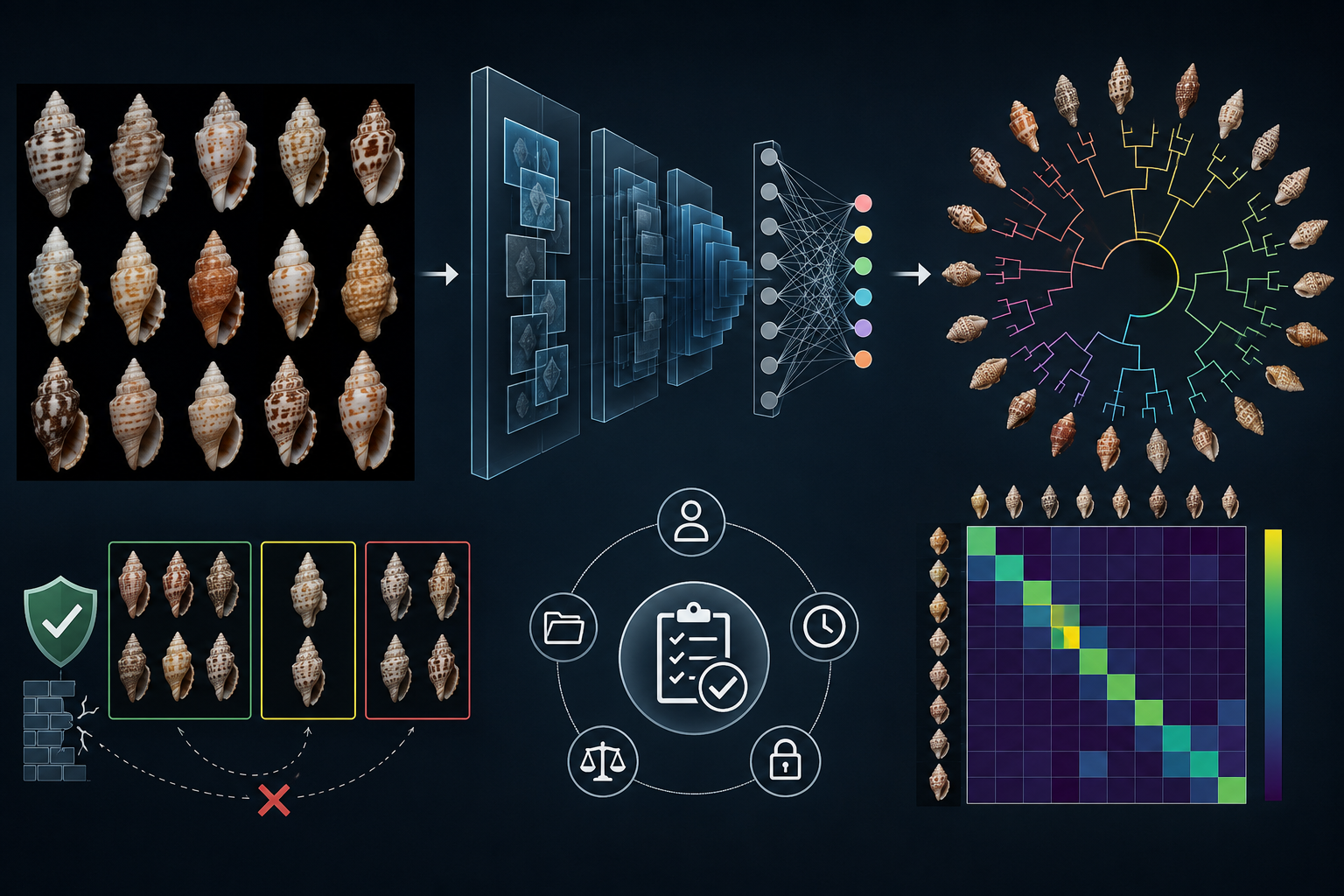
This concentration was most visible in Lienardia and Etrema. All six of the most frequent confusion pairs observed across the two leakage-aware runs were intrageneric: four involved Lienardia and two involved Etrema. The largest combined counts occurred between Lienardia crassicostata and L. roseotincta, and between L. roseotincta and L. rubida. Other recurrent pairs linked L. cincta with L. mighelsi, L. acrolineata with L. cincta, Etrema crassilabrum with E. subauriformis, and E. crassilabrum with E. tenera. Their occurrence in both leakage-aware runs shows that the main confusion structure remained present before and after the technical exclusions.
Several of these relationships were strongly directional rather than balanced exchanges. In the audit-filtered model, L. crassicostata was assigned to L. roseotincta six times, whereas the reverse error occurred once. Five L. rubida images were assigned to L. roseotincta, compared with two errors in the opposite direction. Similarly, all five errors between L. mighelsi and L. cincta involved assignment of the former to the latter, and all five errors between E. subauriformis and E. crassilabrum occurred in the same direction. The confusion pattern therefore cannot be described simply as two species being equally interchangeable in image space. For several pairs, one label attracted predictions from the other more often than it returned them.
This pattern corresponds to the general structure of fine-grained image recognition, in which the classes belong to a shared higher-level category and may differ through relatively localized visual characters. Fine-grained recognition is difficult when differences between classes are small relative to variation within each class [20]. Reviews of automated species identification similarly emphasize that closely related taxa may require attention to restricted diagnostic structures rather than overall object appearance [18]. The present confusion results are consistent with that general problem, because the dominant errors occurred between species already assigned to the same genus rather than between unrelated regions of the label space.
The available results do not identify the individual shell characters responsible for these errors. The classifier may have responded to shell outline, sculpture, aperture, colour pattern or combinations of visible features, but the prediction records do not isolate their contributions. Moreover, not every taxonomically informative character is represented consistently in the standardized images. Previous work on Lienardia has shown that adult shell colour pattern can be interpreted together with protoconch colour and radular morphology [10]. The current classifier cannot use radular evidence, and the protoconch or other small diagnostic structures may not be clearly visible in every image. The observed confusion pairs should therefore be treated as evidence of limited separation in the present shell-image representation, not as evidence that the corresponding species are taxonomically indistinct.
The concentration of errors within genera also limits what can be expected from genus-level routing alone. A Family→Genus classifier could remove some cross-genus alternatives, but it would not resolve an image confused between two species of Lienardia or two species of Etrema; both alternatives would remain available after correct genus assignment. Separate genus-specific classifiers could still be tested because they would operate in a smaller label space, but the current results do not establish that they would improve these particular distinctions. Their value would need to be measured through image-paired comparison with the direct Family→Species model.
The persistent pairs provide more specific development targets than the aggregate error rate alone. Additional curated specimens, consistent apertural and dorsal views, clearer presentation of the protoconch and targeted review of the images involved in the directional confusions could test whether the observed overlap is reduced by better visual coverage. For operational use, predictions within these recurrent pairs may also warrant presentation as ranked alternatives or referral to a lower-confidence decision pathway rather than unconditional single-species assignment.
Natural-distribution accuracy masks unequal species-level reliability
Because the remaining errors were concentrated in particular parts of the species label space, the interpretation of aggregate performance depends on how strongly each species contributes to the evaluation. Under the natural validation distribution, every image contributed once, so species with more held-out images had greater influence on overall accuracy and support-weighted metrics. This evaluation reflects the composition of the available validation cohort, but it does not assign equal importance to all 26 species.
Repeating existing prediction records until each species contributed 43 entries changed the aggregate accuracy from 84.716% to 82.290%. Macro F1 decreased from 83.393% to 82.022%. The lower values under equalized support show that the natural-distribution result was partly sustained by the species that were both more frequently represented and more successfully classified. Once the numerical contribution of every species was made equal, weaker classes exerted greater influence on the aggregate summary.
The effect was not a uniform reduction across all metrics. Equalization decreased macro precision by 2.134 percentage points and macro F1 by 1.371 percentage points, while macro recall increased by 0.694 percentage points. The change therefore represents a redistribution of the relative influence of class-specific true-positive and false-positive outcomes rather than a simple scaling of the natural-distribution scores. No single aggregate metric captures all aspects of that redistribution.
This distinction is well established in multiclass-classification evaluation. Different averaging procedures respond differently to changes in class prevalence and confusion-matrix structure [21]. Support-weighted measures emphasize performance in proportion to the observed number of records, whereas macro-averaged measures give each class the same nominal weight. Research on imbalanced classification consequently recommends that evaluation should not rely exclusively on global accuracy when performance for underrepresented classes is also important [22].
In the present application, neither evaluation perspective is sufficient on its own. The natural-distribution analysis answers how the classifier performed on the validation cohort as it was collected. This is the appropriate primary summary when the intended evaluation target is that observed image mixture. The equal-support analysis addresses a different question: how the aggregate result changes when every included species is given the same number of evaluation records. Its lower accuracy identifies a lack of uniform reliability across the complete species set, even though the classifier remained successful for most validation images.
The equal-support result must also be interpreted according to how it was constructed. It reused predictions already generated for the 458 held-out images and repeated selected records until every species reached the maximum natural support of 43. It introduced neither new specimens nor new model inference. The resulting 1,118 entries therefore do not constitute a larger independent validation set, and record repetition does not increase the amount of empirical evidence available for any species. The analysis is best regarded as a sensitivity assessment of class weighting.
This construction also differs from reporting only the arithmetic mean of the original per-species scores. Because individual prediction records were repeated, the exact equal-support values depend on the composition of the repeated entries. The balanced view is therefore useful for demonstrating how the summary changes under equal record support, but it should not replace the natural image-level results, macro averages or original per-species metrics.
For operational reporting, the natural-distribution accuracy should remain the principal estimate of performance on the observed validation cohort. It should, however, be presented together with macro metrics, species-level scores and confusion patterns. This combination distinguishes a model that performs well for many images from one that performs consistently across all included species. It also prevents strong results for well-represented classes from obscuring weaker reliability in smaller or more difficult classes.
The dependence of the summary result on class weighting is also relevant to model selection. A configuration selected solely by overall accuracy need not be the configuration that provides the most even performance across the species label space. The basis on which the final Clathurellidae model was retained must therefore be considered separately from the highest individual metric observed during the configuration search.
The final model was selected by protocol completion rather than maximum observed accuracy
The differences between natural-distribution and equal-support metrics also show that model selection depends on the criterion being prioritized. In the original-partition configuration search, no single run produced the highest value for every reported metric, and the configuration subsequently carried forward was not the numerically strongest original-split model.
The audit-filtered classifier was designated the final evaluated model because it was trained on the leakage-aware partition after completion of the predefined data-audit workflow. Its selection therefore reflects protocol completion and dataset governance rather than maximum observed accuracy. This distinction is important when interpreting the model as the final output of the study, but it does not imply that its training configuration was established as statistically optimal.
Implications for deployment and dataset governance
Selecting the final classifier as the output of a controlled data and evaluation protocol has consequences for deployment. The deployable artifact should not be limited to the serialized neural network. It should remain associated with the exact taxonomic label mapping, preprocessing configuration, training-data revision, partition manifests, audit decisions and evaluation results from which it was produced. Separating the model from these elements would make it difficult to determine which species concept, image transformation or dataset revision a prediction represents.
The model must also be presented according to its actual label space. It is a closed 26-species classifier rather than a classifier for every member of Clathurellidae. Its output identifies the most strongly supported alternative among the 26 included classes; it does not establish that an input belongs to one of those species. This distinction is central to open-set recognition, where operational inputs may belong to classes that were absent during training [25]. Deployment should therefore distinguish a prediction within the supported label space from confirmation of a family-wide species identification.
The interface should likewise reflect the unequal reliability of the included classes. For recurrent confusion pairs, presenting ranked alternatives may be more informative than displaying only the highest scoring species. A lower-resolution result, such as genus-level assignment, or an unresolved outcome may also be preferable when the available evidence is insufficient for a reliable species decision. The present study did not evaluate probability calibration or derive abstention thresholds, so such decision rules would require separate validation and should not be inferred directly from the existing softmax scores.
Dataset governance is equally important when the model is updated. New images should retain persistent identifiers, source information, specimen- or listing-group membership and content hashes. They should be added through a new dataset revision rather than silently replacing the records used for the current model. Known views of the same specimen and recognized duplicates must continue to share a partition, and audit evidence should be regenerated whenever the image content, preprocessing procedure, taxonomic mapping or embedding configuration changes.
Taxonomic changes require similar version control. A newly recognized synonym may require only an update to the mapping between published and accepted names, whereas a change in species circumscription may alter the meaning of one or more model classes and require reconstruction of the affected dataset. Recording the taxonomic source and its retrieval date makes it possible to distinguish a nomenclatural update from a change in the biological definition of a class.
The retained manifests, fingerprints and reversible audit decisions provide a suitable basis for this form of governance. They allow a future dataset revision to be compared with the version used for the present model and make it possible to identify which records were added, removed, relabelled or technically reprocessed. The audit can then remain a screening stage within the update process, while statistical flags, technical failures and human decisions continue to be stored as separate forms of evidence rather than being collapsed into an undocumented deletion.
These practices are consistent with proposals for structured dataset and model documentation. Datasheets for datasets emphasize documentation of dataset motivation, composition, collection, preprocessing and maintenance [23], while model cards provide a framework for recording intended use, evaluation conditions and known differences in performance across relevant groups [24]. For the present classifier, such documentation should identify the supported species, dataset and taxonomy revision, preprocessing fingerprint, evaluation cohort and species-level performance profile.
A replacement model should consequently be evaluated as a new governed artifact rather than accepted solely because it improves one aggregate metric. Comparison should use a declared evaluation cohort and report changes in macro, weighted and species-level performance, together with any new or resolved confusion patterns. These deployment safeguards define how the present model can be used and updated, but they do not remove the limitations of the available validation evidence, which are considered in the following section.
Limitations of the present evaluation
The governance requirements described above define how the model and its supporting data should be maintained, but they do not expand the empirical evidence available for judging performance. The reported results should therefore be interpreted as an internal evaluation of one defined dataset, model architecture and taxonomic label space rather than as a complete estimate of performance across Clathurellidae or across all possible deployment conditions.
The most important limitation is the absence of an independent test set. The 458-image leakage-aware validation partition was used to monitor model fitting and was also the source of the post-training predictions reported as the principal evaluation. It was protected from the data audit and from direct training, but it was not an untouched external test cohort because validation performance informed the training process through early stopping. The reported metrics are consequently held-out validation results, not estimates obtained from specimens or image sources that were completely independent of model development.
The experimental series also provides limited information about variability between training runs. Most fine-tuning configurations were evaluated once, and the principal leakage-aware and audit-filtered conditions were each represented by a single run. Their training seeds differed, and deterministic TensorFlow execution was not enabled. Small differences between models therefore cannot be separated reliably into effects of dataset composition, optimization settings and stochastic training variation. Repeated training with fixed sets of seeds would be needed to estimate the stability of the reported comparisons.
Uncertainty is especially relevant at species level. Individual validation supports ranged from 7 to 43 images, and no confidence intervals or repeated-split variability estimates were calculated for the species-specific metrics. Scores based on the smallest classes may therefore change substantially when additional specimens are evaluated. More generally, predictive-performance estimates derived from limited samples can have considerably larger uncertainty than a single reported score suggests [27]. The ranked species results should be treated as evidence from the present cohort rather than as precise population-level performance estimates.
Taxonomic and geographic coverage was also restricted by image availability. The classifier included 26 species from eight genera, selected because they met the minimum image threshold and could be assigned to accepted names. This set is neither a random sample nor an exhaustive representation of Clathurellidae. Several genera were represented by only one eligible species, while Lienardia accounted for most of the available records. The results therefore describe discrimination among the included labels and cannot be extrapolated directly to unrepresented species, genera or populations.
The images originated from multiple online repositories, specialist collections and commercial sources and were transformed into standardized, shell-centred records. No independently collected deployment cohort was evaluated. Performance may change when the distribution of image sources, specimen preservation, viewing angles, backgrounds, geographic populations or photographic conditions differs from that represented during model development. Such changes constitute forms of dataset shift, under which the relationship between the development data and later operational data may no longer remain constant [26]. The present evaluation does not quantify the magnitude of any such shift.
Leakage control was necessarily limited to relationships that could be identified from the retained source, specimen, listing and duplicate information. Group-aware partitioning kept known related records together, but the available metadata cannot prove that every repeated specimen, derivative image or cross-source duplicate was recognized. Undetected dependencies between training and validation images therefore cannot be excluded completely.
The model was evaluated only from standardized shell imagery. Characters that were absent or inconsistently visible—including radular morphology, soft anatomy, protoconch details, locality and molecular evidence—could not contribute to the prediction. Similarly, the study measured recovery of the accepted operational labels but did not test whether those labels represent phylogenetically or anatomically homogeneous species concepts. Model errors and successes should therefore not be interpreted as direct evidence for or against the underlying taxonomy.
Finally, the deployment controls proposed in the preceding section remain prospective. The study did not evaluate confidence calibration, rejection thresholds, abstention behaviour or recognition of species outside the 26-class label space. Open-set performance cannot be inferred from closed-set validation [25], and the existing softmax probabilities have not been shown to provide reliable decision thresholds for accepting or withholding a species identification.
These limitations do not invalidate the comparison of the evaluated workflows, but they restrict the scope of the conclusions. The present model provides a reproducible internal benchmark for the selected species and image corpus. Establishing broader operational validity will require repeated training, independent evaluation material, expert review of unresolved audit candidates and direct testing under the image conditions expected during deployment.
Priorities for further validation and model development
The limitations of the present evaluation define a sequence of priorities for the next development stage. The immediate objective should not be to increase aggregate accuracy through additional configuration searches, but to determine whether the observed performance patterns remain stable under repeated training and more independent evaluation conditions.
Repeated evaluation under the leakage-aware protocol
The leakage-aware and audit-filtered conditions should first be repeated using a predefined set of training seeds. Reporting the mean, dispersion and range of the resulting metrics would distinguish stable species-level behaviour from differences attributable to model initialization and training order. Where dataset size permits, additional group-aware partitions could be evaluated to determine whether the principal findings depend strongly on one particular allocation of specimens to training and validation. This is especially important for species represented by small validation cohorts, for which a single score may have considerable sampling uncertainty [27].
Independent source- and specimen-level testing
The strongest next validation step would be a locked test collection assembled independently of model fitting, audit threshold development and configuration selection. Its images should originate from specimens, listings and, where possible, image sources not represented in the development partitions. Recording source and geographic provenance would also allow performance to be examined across acquisition conditions rather than only as one pooled result. Such an evaluation would provide a more direct test of robustness to dataset shift [26].
Targeted expansion of weak species and confusion pairs
Additional data collection should be guided by the observed error structure rather than by class counts alone. Priority should be given to species with low or unstable performance and to the recurrent confusion pairs within Lienardia and Etrema. New material should preferably add independent specimens, geographic variation and consistently documented diagnostic views, including apertural, dorsal and protoconch views where these characters are visible. Fine-grained recognition studies emphasize that additional images are most useful when they increase the coverage of diagnostically relevant variation rather than merely duplicate already common appearances [18], [20].
The persistent intrageneric errors also justify a direct comparison between the current Family→Species classifier and genus-specific species classifiers for Lienardia and Etrema. Such models should be evaluated through image-paired replay on the same held-out records, including the effect of any preceding genus-routing decision. A smaller within-genus label space may alter the confusion structure, but improvement should be demonstrated empirically rather than assumed from the hierarchy.
Sensitivity analysis of the audit thresholds
The statistical audit can be examined further without requiring taxonomic review of the complete training corpus. A targeted sensitivity study could compare a blinded sample of the highest-ranked disagreements with a randomly selected control sample of unflagged images. This would not provide complete ground truth for all 1,837 training records, but it could indicate whether the present conjunctive thresholds are so conservative that strongly questionable labels remain systematically below the exclusion boundary. Any expert decisions produced by such a study should remain separate from the original audit evidence and be stored as a new, reversible decision revision.
Confidence-aware and open-set operation
Further model development should also address how predictions are presented when the evidence is insufficient for an unconditional species assignment. A separate calibration dataset could be used to evaluate whether predicted probabilities correspond to observed correctness and to define thresholds for returning a ranked species list, a genus-level result or an unresolved outcome. Open-set experiments should additionally include Clathurellidae species outside the current 26-class label space, because closed-set performance does not establish that the model can recognize an unsupported species as unknown [25].
Predefined criteria for model replacement
Future versions should be accepted through declared comparison criteria rather than through the highest result from an exploratory run. A candidate replacement should be evaluated on the same locked cohort and compared in terms of overall, macro and species-level performance, recurrent confusion pairs, calibration and open-set behaviour. Improvements in one aggregate score should be considered together with any deterioration among weak or operationally important species.
Each accepted revision should retain its dataset inventory, taxonomic mapping, preprocessing and model fingerprints, audit provenance and evaluation report. Structured dataset and model documentation provides an appropriate mechanism for recording these changes [23], [24].
These priorities would extend the present study from a controlled internal benchmark toward an independently validated identification system. They would also preserve the central distinction established by the current workflow: improvements should result from stronger evidence, broader coverage and reproducible evaluation, rather than from simplifying the dataset or selecting a favourable single run.
Conclusion
This study establishes a reproducible workflow for species-level shell-image classification within a defined subset of Clathurellidae. Its principal contribution is not a single maximum performance value, but the integration of taxonomic normalization, specimen- and duplicate-aware partitioning, conservative training-data audit and traceable production-model evaluation within one controlled pipeline.
The resulting classifier showed that standardized shell photographs contain sufficient visual information for reliable recovery of many of the 26 included species, while also revealing substantial differences in species-level diagnosability. The remaining errors were concentrated mainly among closely related species within Lienardia and Etrema, demonstrating that the principal unresolved challenge is fine-grained intrageneric discrimination rather than broad separation across the complete label space.
The data audit further showed that statistical disagreement should not be treated automatically as evidence of an incorrect label. Retaining ambiguous records while removing directly unusable images preserved difficult biological variation without allowing technical defects to remain in the production dataset. The audited model should therefore be understood as the final output of a governed workflow rather than as a statistically proven optimum among all possible model configurations.
The present classifier is consequently a controlled benchmark for the included species, not a complete identification system for Clathurellidae. Broader operational use will require independent specimen-level testing, repeated training, expansion of weakly represented taxa, targeted investigation of persistent confusion pairs and explicit handling of species outside the current label space. Maintaining the same partitioning, audit and provenance controls during those extensions will be essential if future performance improvements are to remain scientifically interpretable.
References
- [1] N Puillandre et al. Starting to unravel the toxoglossan knot: molecular phylogeny of the ‘turrids’ (Neogastropoda: Conoidea). Molecular Phylogenetics and Evolution 47(3): 1122–1134 (2008)
- [2] N Puillandre et al. The dragon tamed? A molecular phylogeny of the Conoidea (Gastropoda). Journal of Molluscan Studies 77(3): 259–272 (2011)
- [3] Ph Bouchet et al. A new operational classification of the Conoidea (Gastropoda). Journal of Molluscan Studies 77(3): 273–308 (2011)
- [4] MolluscaBase / WoRMS. Clathurellidae H. Adams & A. Adams, 1858. MolluscaBase / WoRMS (last accessed 26-Jul-2026)
- [5] Ph Kerremans. Source-Aware Training Improves Robustness in Leakage-Aware CNN Species Classification of Morum Röding, 1798 (Gastropoda: Harpidae). IdentifyShell (2026)
- [6] Ph Kerremans. DINOv3 Improves Class-Balanced Recovery but Not Global Accuracy in Harpa Shell Classification. IdentifyShell (2026)
- [7] Ph Kerremans. Conservative Statistical Label Curation for Leakage-Aware CNN Species Classification of Harpa Röding, 1798. IdentifyShell (2026)
- [8] J Abdelkrim et al. Exon-Capture-Based Phylogeny and Diversification of the Venomous Gastropods (Neogastropoda, Conoidea). Molecular Biology and Evolution 35(10): 2355–2374 (2018)
- [9] J E Uribe, R Zardoya and N Puillandre. Phylogenetic relationships of the conoidean snails (Gastropoda: Caenogastropoda) based on mitochondrial genomes. Molecular Phylogenetics and Evolution 127: 898–906 (2018)
- [10] G Rosenberg and P Stahlschmidt. A new species of Lienardia (Gastropoda: Conoidea) from the Philippines and the Spratly Islands. Proceedings of the Academy of Natural Sciences of Philadelphia 161(1): 105–115 (2011)
- [11] G Fassio et al. An assessment of Raphitoma and allied genera (Neogastropoda: Raphitomidae). Journal of Molluscan Studies 85(4) (2019)
- [12] Ph Bouchet at al. Revised Classification, Nomenclator and Typification of Gastropod and Monoplacophoran Families. >Malacologia 61(1–2): 1–526 (2017)
- [13] S Kapoor and A Narayanan. Leakage and the reproducibility crisis in machine-learning-based science. Patterns 4(9): 100804 (2023)
- [14] D R Roberts et al. Cross-validation strategies for data with temporal, spatial, hierarchical, or phylogenetic structure. Ecography 40(8): 913–929 (2017)
- [15] B Barz and J Denzler. Do We Train on Test Data? Purging CIFAR of Near-Duplicates. >Journal of Imaging 6(6): 41 (2020)
- [16] C G Northcutt, L Jiang and I L Chuang. Confident Learning: Estimating Uncertainty in Dataset Labels. Journal of Artificial Intelligence Research 70, 1373–1411 (2021)
- [17] B Frénay and M Verleysen. Classification in the Presence of Label Noise: A Survey. IEEE Transactions on Neural Networks and Learning Systems, 25(5), 845–869 (2014)
- [18] J Wäldchen and P Mäder. Machine Learning for Image Based Species Identification. Methods in Ecology and Evolution 9:2216–2225 (2018)
- [19] G Van Horn et al. The iNaturalist Species Classification and Detection Dataset.. In Proceedings of the IEEE/CVF Conference on Computer Vision and Pattern Recognition (CVPR), 8769–8778. (2018)
- [20] X-S Wei et al. Fine-Grained Image Analysis With Deep Learning: A Survey. IEEE Transactions on Pattern Analysis and Machine Intelligence, 44(12), 8927–8948 (2022)
- [21] M Sokolova and G Lapalme. A systematic analysis of performance measures for classification tasks. Information Processing & Management 45(4): 427–437 (2009)
- [22] H He and E A Garcia. Learning from Imbalanced Data. IEEE Transactions on Knowledge and Data Engineering 21(9): 1263–1284 (2009)
- [23] T Gebru et al. Datasheets for Dataset. Communications of the ACM 64(12): 86–92 (2021)
- [24] M Mitchell et al. Model Cards for Model Reporting. Proceedings of the Conference on Fairness, Accountability, and Transparency 220–229. (2019)
- [25] W J Scheirer et al. Toward Open Set Recognition. IEEE Transactions on Pattern Analysis and Machine Intelligence 35(7): 1757–1772 (2013)
- [26] J G Moreno-Torres et al. A unifying view on dataset shift in classification. Pattern Recognition 45(1): 521–530 (2012)
- [27] G Varoquaux . Cross-validation failure: Small sample sizes lead to large error bars. NeuroImage 180: 68–77 (2018)
Supplement
Table S1. Taxonomic composition of the Clathurellidae dataset
| Genus | Species |
Initial total |
Training before audit |
Held-out validation |
Technical exclusions |
Final audited training |
Final audited total |
|---|---|---|---|---|---|---|---|
| Clathurella | Genus subtotal | 114 | 91 | 23 | 0 | 91 | 114 |
| Clathurella colombi | 60 | 48 | 12 | 0 | 48 | 60 | |
| Clathurella grayi | 54 | 43 | 11 | 0 | 43 | 54 | |
| Corinnaeturris | Genus subtotal | 60 | 48 | 12 | 0 | 48 | 60 |
| Corinnaeturris leucomata | 60 | 48 | 12 | 0 | 48 | 60 | |
| Etrema | Genus subtotal | 501 | 401 | 100 | 0 | 401 | 501 |
| Etrema crassilabrum | 122 | 98 | 24 | 0 | 98 | 122 | |
| Etrema leukospiralis | 114 | 91 | 23 | 0 | 91 | 114 | |
| Etrema scalarina | 91 | 73 | 18 | 0 | 73 | 91 | |
| Etrema spurca | 68 | 54 | 14 | 0 | 54 | 68 | |
| Etrema subauriformis | 65 | 52 | 13 | 0 | 52 | 65 | |
| Etrema tenera | 41 | 33 | 8 | 0 | 33 | 41 | |
| Lienardia | Genus subtotal | 1,402 | 1,122 | 280 | 9 | 1,113 | 1,393 |
| Lienardia acrolineata | 36 | 29 | 7 | 0 | 29 | 36 | |
| Lienardia cincta | 156 | 125 | 31 | 0 | 125 | 156 | |
| Lienardia coccinea | 39 | 31 | 8 | 0 | 31 | 39 | |
| Lienardia crassicostata | 122 | 98 | 24 | 0 | 98 | 122 | |
| Lienardia fallax | 83 | 66 | 17 | 2 | 64 | 81 | |
| Lienardia grandiradula | 69 | 55 | 14 | 0 | 55 | 69 | |
| Lienardia mighelsi | 115 | 92 | 23 | 0 | 92 | 115 | |
| Lienardia nigrotincta | 69 | 55 | 14 | 1 | 54 | 68 | |
| Lienardia planilabrum | 97 | 78 | 19 | 1 | 77 | 96 | |
| Lienardia purpurata | 112 | 90 | 22 | 0 | 90 | 112 | |
| Lienardia roseotincta | 213 | 170 | 43 | 2 | 168 | 211 | |
| Lienardia rubida | 211 | 169 | 42 | 3 | 166 | 208 | |
| Lienardia tricolor | 80 | 64 | 16 | 0 | 64 | 80 | |
| Nannodiella | Genus subtotal | 55 | 44 | 11 | 0 | 44 | 55 |
| Nannodiella vespuciana | 55 | 44 | 11 | 0 | 44 | 55 | |
| Paraclathurella | Genus subtotal | 46 | 37 | 9 | 0 | 37 | 46 |
| Paraclathurella gracilenta | 46 | 37 | 9 | 0 | 37 | 46 | |
| Pseudoetrema | Genus subtotal | 60 | 48 | 12 | 0 | 48 | 60 |
| Pseudoetrema crassicingulata | 60 | 48 | 12 | 0 | 48 | 60 | |
| Strombinoturris | Genus subtotal | 57 | 46 | 11 | 0 | 46 | 57 |
| Strombinoturris crockeri | 57 | 46 | 11 | 0 | 46 | 57 | |
| Complete dataset | 2,295 | 1,837 | 458 | 9 | 1,828 | 2,286 | |
Table S2. Training images assigned to technical quarantine
A. Records omitted from the audited training dataset
| Species assigned in dataset | Manifest image identifier | Partition | Audit decision |
|---|---|---|---|
| Lienardia fallax | 335852430843009038_Y0.jpg |
Training | Technical quarantine |
| Lienardia fallax | m4768180412403530928_Y0.jpg |
Training | Technical quarantine |
| Lienardia nigrotincta | 3437173243763469873_Y0.jpg |
Training | Technical quarantine |
| Lienardia planilabrum | 816313205947210425_Y0.jpg |
Training | Technical quarantine |
| Lienardia roseotincta | 2791227936854020414_Y0.jpg |
Training | Technical quarantine |
| Lienardia roseotincta | 830303995760804829_Y0.jpg |
Training | Technical quarantine |
| Lienardia rubida | 3978597690630700944_Y0.jpg |
Training | Technical quarantine |
| Lienardia rubida | 5920892927597979328_Y0.jpg |
Training | Technical quarantine |
| Lienardia rubida | 6261086353659132473_Y0.jpg |
Training | Technical quarantine |
| Total | Training | 9 images | |
B. Aggregate technical-exclusion reasons
| Recorded exclusion reason | Images | Percentage of exclusions |
|---|---|---|
| Identification label or documentation instead of a shell specimen | 6 | 66.7% |
| No shell present | 1 | 11.1% |
| Wrong object depicted | 1 | 11.1% |
| Otherwise unusable for visual model training | 1 | 11.1% |
| Total | 9 | 100.0% |