Species Delimitation as Human-Led Triage: A Stability-Aware Embedding Benchmark with COX1 Validation in Cone Snails (Gastropoda: Conidae) from Maio, Cape Verde
Published on: March 2026
Abstract
Digitized shell-image datasets assembled from museum, collector, dealer, and online sources are increasingly valuable for biodiversity research, but they are also highly heterogeneous and often contain taxonomic inconsistency, label noise, and uneven image quality. In such settings, conventional classifier performance is not sufficient to assess whether a dataset is internally coherent or taxonomically defensible. Here, a human-led, embedding-based benchmark for species-delimitation support and label-noise triage in heterogeneous collector imagery is presented, using Conus from Maio, Cabo Verde, as a geographically constrained case study. The workflow is designed explicitly as decision support rather than automated taxonomy. Images are embedded into a learned phenotype space and evaluated using three interpretable diagnostics: within-species cohesion, outlier burden, and pairwise interference. To make these signals reproducible and defensible, uncertainty estimates are attached through bootstrap resampling and repeated-run stability metrics, including worst-rank frequency and Top-10 persistence.
The results show marked heterogeneity among named taxa. Some species form compact and stable groups in embedding space, whereas others are consistently diffuse, outlier-rich, or entangled with specific rival taxa. Bootstrap analyses demonstrate that several weak clusters and interference pairs recur persistently across perturbations, indicating that the workflow captures not only point estimates of structure but also the stability of candidate problem cases. Mitochondrial COX1 data were incorporated as an orthogonal validation layer. Species-level and pairwise comparisons showed partial rather than complete concordance between mitochondrial and embedding-based structure: some close embedding relationships were supported by low interspecific COX1 distance, whereas others remained discordant despite substantial mitochondrial separation. These results indicate that, within the represented Maio/Cape Verde comparison set, embedding-based confusion contains both biologically plausible and non-concordant components.
The main value of the framework is methodological rather than taxonomic. It provides a reproducible benchmark for identifying compact taxa, unstable taxa, persistent outliers, and problematic species pairs, while preserving final taxonomic interpretation as a human-led task. In this role, embeddings function as a structured review layer and COX1 as an external plausibility signal, together supporting a scalable and uncertainty-aware workflow for species-delimitation triage in heterogeneous natural-history image datasets, although the present benchmark was evaluated only on the represented Maio/Cape Verde Conus comparison set.
Introduction
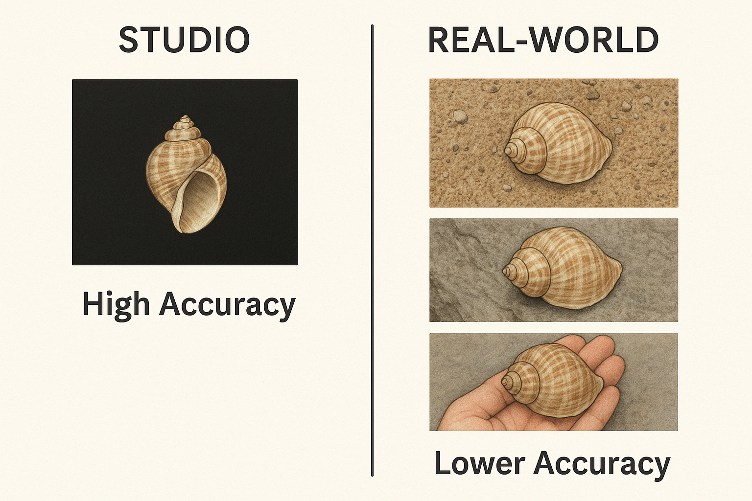
Digitized biodiversity imagery has expanded rapidly through museum programs, private collections, dealer archives, and citizen-science platforms, but the resulting datasets are often heterogeneous in lighting, background, scale, camera optics, and viewpoint. In biodiversity vision, this heterogeneity is compounded by long-tailed class distributions and fine-grained visual similarity between taxa, making annotation quality a central bottleneck rather than a secondary nuisance. More broadly, data-centric AI work has emphasized that model performance is frequently limited by data quality, maintenance, and reliability, and large-scale benchmark analyses have shown that even widely used test sets can contain enough label errors to destabilize evaluation and model ranking [18].
This problem is especially acute for collector and museum imagery. Labels may reflect historical synonymies, local naming conventions, outdated taxonomy, variable expert thresholds, or simple identification mistakes. In such settings, conventional supervised learning is useful, but it can also absorb and propagate label noise rather than expose it. As a result, a high-performing classifier does not necessarily imply a clean dataset, and marginal gains in top-1 accuracy may say little about whether a collection has become more internally consistent or more taxonomically defensible. Recent work on label issue detection and training-dynamics analysis has reinforced this point by treating label quality as an explicit target of analysis rather than a hidden assumption [18].
Embedding-based analysis offers a different route. Instead of asking only whether an image is assigned the correct name by a classifier, embedding methods treat image representations as a quantitative phenotype space that can be interrogated for internal consistency, anomalous specimens, and cross-label overlap. General-purpose visual representations derived from large-scale contrastive or self-supervised training, including CLIP and DINOv2, have made this strategy increasingly practical across domains. In biodiversity and delimitation-adjacent work, embeddings have been used not just for recognition, but for neighborhood analysis, exploratory morphospaces, clustering behavior, and expert-in-the-loop interpretation of visually confusable groups [19].
However, embedding geometry alone is not enough. For a triage system to be scientifically useful, it must be reproducible, uncertainty-aware, and embedded within a human review process. A practical benchmark therefore needs more than a single set of point estimates: it needs metrics that remain informative under resampling, rankings that are stable across repeated runs, and outputs that can be audited by domain experts. This requirement is consistent with recent natural-history collections work showing that repeated computer-vision runs, coupled to expert inspection and selective genetic verification, can identify likely mislabels at scale and turn stochastic model behavior into a reproducible curation signal [20].
The cone snails of Cabo Verde provide an especially relevant testbed for such a benchmark. Cabo Verde is a marine endemism hotspot, and its cone-snail fauna is remarkable for high endemicity at small spatial scales; many taxa are restricted to single islands and often to narrow stretches of coastline or even individual bays. Molecular work has shown that the radiation is evolutionarily recent and geographically structured, while shell coloration and patterning can be affected by homoplasy and may not map cleanly onto currently used taxonomic names [7]. In large-shelled Cabo Verde taxa, mitochondrial phylogenies have also shown that visually defined species boundaries do not always correspond neatly to genetic clades, underscoring the difficulty of image-only identification in this group [21, 22].
Within that broader system, Maio is a useful case-study anchor because it combines constrained geography with a taxonomically challenging morphospecies assemblage. This makes it possible to ask a focused question: when images are embedded into a learned phenotype space, do some named species form compact and stable clusters, while others remain heterogeneous, outlier-rich, or entangled with specific rival taxa? Framed this way, the task is not automatic species delimitation in the strict taxonomic sense, but human-led dataset auditing and decision support for curation. That distinction is important, because species delimitation remains a hypothesis-testing enterprise that integrates morphology, geography, genetics, and expert judgment rather than a direct output of any single algorithm [23].
Mitochondrial DNA provides an additional, orthogonal signal for this workflow. COX1-based barcoding has long been valuable for animal identification, and mitogenomic work in Cabo Verde Conus provides an independent view of lineage structure that can be used to assess whether embedding-based confusion reflects plausible biological proximity or a likely imaging/label artifact. At the same time, mitochondrial markers cannot be treated as a taxonomic oracle, because mito-nuclear discordance is widespread in animals and discordant cases may arise from introgression, incomplete lineage sorting, or other evolutionary processes [28]. For that reason, DNA is best used here as a validity signal in aggregate, not as an automatic split/lump mechanism [24]
Against this background, the present study introduces a human-led, embedding-based benchmark for label-noise triage in collector imagery. Its primary thesis is that reproducible curation can be improved by quantifying three interpretable diagnostics in embedding space—cohesion, outlier burden, and pairwise interference—and by attaching explicit stability estimates to those diagnostics through bootstrap resampling. Its secondary thesis is methodological: machine-assisted delimitation in this setting should be treated as decision support, not automated relabeling or automated taxonomy. Using Conus from Maio, Cape Verde, as a geographically constrained case study, the analysis evaluates whether embedding structure recovers meaningful morpho-species patterns, which labels and label pairs are consistently flagged, and whether mitochondrial DNA provides an orthogonal concordance signal for the most problematic cases.
Related Work
A first relevant body of literature comes from data-centric AI and learning with noisy labels. This work argues that data quality, label maintenance, and error auditing are often more consequential than incremental changes in model architecture. Confident Learning formalized label-error detection as estimation of the joint distribution between noisy and latent labels, while dataset cartography used training dynamics to identify easy, ambiguous, and hard-to-learn examples, with the latter often enriched for annotation problems. Benchmark studies have further shown that label errors are not confined to obscure datasets: they are widespread enough in common test sets to alter measured performance and benchmark rankings [18, 50].
A second relevant thread concerns representation learning as a substrate for robust image analysis. CLIP demonstrated that contrastive image-text pretraining can yield transferable visual representations across many downstream tasks, while DINOv2 showed that large-scale self-supervised pretraining can produce strong all-purpose visual features without task-specific labels. In biodiversity imaging, these developments matter because the operating regime is usually fine-grained, imbalanced, and noisy rather than clean and evenly sampled. The iNaturalist benchmark made this explicit by framing biodiversity recognition as a real-world challenge characterized by severe class imbalance and high visual similarity among taxa [17]. More recent work has also suggested that foundation-model embeddings can be paired with neighborhood-based reliability estimates to improve robustness under noisy labels [18].
A third line of work is more directly aligned with embedding-first biodiversity analysis. In planktic foraminifera, deep metric learning has been used to construct an explicit morphological appearance space in which distances are interpretable, unseen taxa can be clustered, and experts can interact with a low-dimensional morphospace rather than only consume classifier outputs [25]. Follow-on work aligned visual embeddings with independently embedded genetic sequences, showing that image space and sequence space can be brought into correspondence and used jointly, especially for rare classes. These studies are important not because they “solve” species delimitation, but because they show a defensible pattern for treating embeddings as scientific objects in their own right: spaces to be inspected, compared, and validated, not just hidden layers inside a classifier.
At the level of collection curation, recent natural-history work provides perhaps the closest operational precedent for the present study. Hollister et al. [20] applied a computer-vision pipeline to a large Lepidoptera collection, ran the pipeline repeatedly, and prioritized specimens that were flagged consistently across runs. Experts then reviewed the flagged subset and used selective genetic verification, demonstrating that repeated-run instability can be turned into a reproducible curation signal rather than dismissed as mere stochastic noise. This logic closely matches the present benchmark’s emphasis on stability: a label or pair is more actionable when it is repeatedly problematic under perturbation, not only when it appears extreme in a single run.
The specific diagnostics used here also connect to established quantitative traditions. Cohesion is closely related to cluster compactness and separation, as captured in silhouette-style reasoning [26]. Outlier burden is related to local density deviation, as formalized by Local Outlier Factor [51]. Pair-interference corresponds to cross-label neighborhood overlap or class-level confusion, which has been discussed both in embedding comparison work and in class-based analysis of embedding visualizations. What distinguishes the present study is not the invention of entirely new mathematical primitives, but their combination into a benchmark for human-led triage, with uncertainty and resampling stability treated as first-class outputs.
Finally, this work sits within the broader context of integrative taxonomy and species delimitation, where multiple evidence streams are brought together to evaluate lineage hypotheses. Reviews in systematics have long argued that delimitation is not reducible to a single operational criterion and that morphology, molecules, geography, and ecology must be interpreted jointly [23]. This matters acutely in Cabo Verde Conus. Molecular studies of the radiation have revealed strong geographic structure, recent diversification, and cases where shell-based assignments and mitochondrial lineages do not correspond cleanly, while conservation syntheses have emphasized the extreme spatial restriction and endemism of many Cape Verde cone snails. In that context, a human-led embedding benchmark is best understood as an aid to triage and hypothesis prioritization: it helps identify which labels, specimens, and species pairs most deserve expert scrutiny, while leaving formal taxonomic decisions to integrative follow-up [23].
Materials and methods
Data acquisition
Shell images were acquired from more than 30 online resources, including specialized shell-collecting websites, institutional and university collections, biodiversity repositories, and online marketplaces. Major sources included GBIF, Malacopics, Femorale, Thelsica, and a previously published shell image dataset for artificial intelligence applications [6]. Most sources were harvested during the period 2020–2024. In addition, six selected sources were monitored continuously and scraped monthly using automated scripts to retrieve newly available records.
Images were included only when sufficient metadata (scientific name at minimum) were available for downstream curation and analysis. At minimum, the retrieved metadata comprised the reported scientific name and source URL; when available, additional metadata such as locality, collector, specimen identifier, and shell size were also captured.
Data acquisition was performed either through direct download facilities provided by the source websites or, when such facilities were unavailable, through custom web-scraping workflows. These scrapers were developed in Python 3.8 using the Scrapy framework (version 2.11.2) to extract shell images and associated metadata. All retrieved records were stored in a MySQL database prior to subsequent taxonomic standardization, quality control, deduplication, and preprocessing. Duplicate detection was performed at multiple levels, including repeated source URLs and repeated source-specific record identifiers present in the metadata.
DNA sequence data were retrieved programmatically using Biopython [5]. Sequence acquisition targeted records assigned to the genus Conus. To match the geographic scope of the image-based dataset, a selection was subsequently applied to retain only specimens with locality information indicating Cape Verde. The resulting subset was used for downstream molecular analyses and comparison with the morphology-based results.
The Conus dataset from Maio, Cape Verde
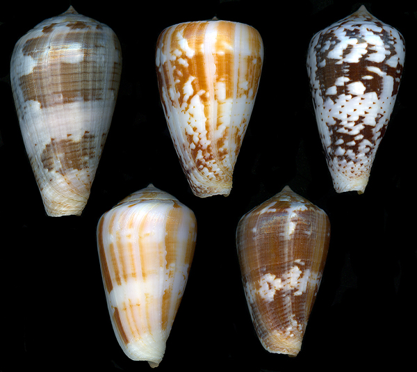
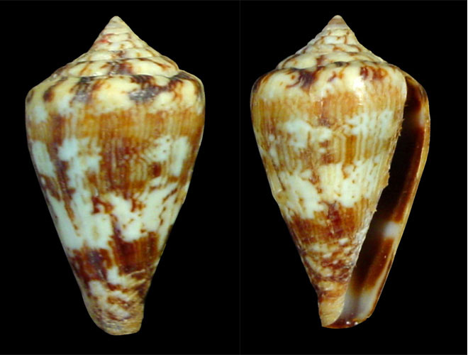
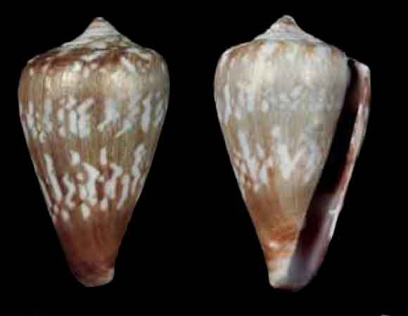
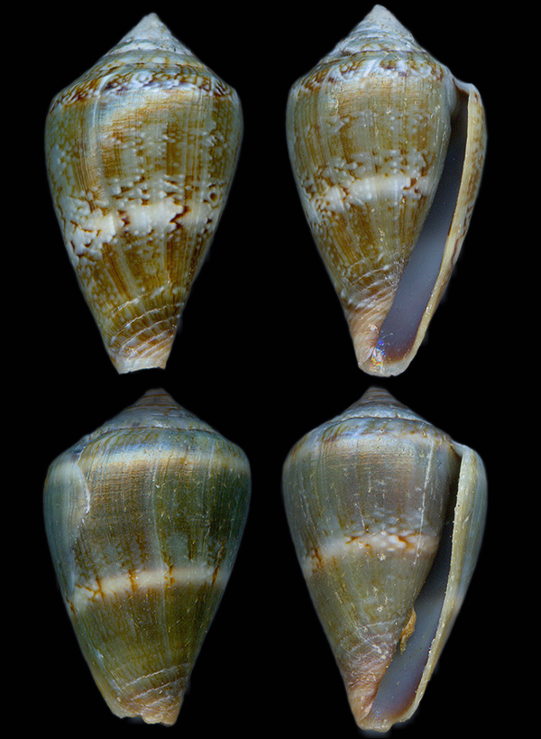
The image dataset comprised all available images of Conus shells endemic to Maio Island, together with images of Conus species recorded from other Cape Verdean islands and considered potentially present on Maio Island. Only images linked to a scientific name matching either an accepted species or a synonym were included. Taxonomic validation was performed using WoRMS and MolluscaBase, and the classification of Tenorio et al. [7] was followed to assign synonyms to the accepted species used in the present study. The full list of included taxa, including accepted names and synonyms, is provided in Table 1.
Table 1. Maio Conus
| Original name | Accepted name | Locality | # Images |
|---|---|---|---|
| Africonus angeluquei M. Tenorio, Abalde & Zardoya, 2018 (AphiaID 1251269) | C. perrineae | Maio | 9 |
| Conus (Kalloconus) atlanticoselvagem Afonso & M. Tenorio, 2004 (AphiaID 847730) | C. trochulus | Between Maio and Boa Vista | 24 |
| Conus navarroi calhetae Rolán, 1990 (AphiaID 428460) | C. calhetae | Maio | 24 |
| Africonus cazalisoi Cossignani & Fiadeiro, 2018 (AphiaID 1074673) | C. trochulus | Maio | 6 |
| Conus claudiae Tenorio & Afonso, 2004 (AphiaID 225104) | C. galeao | Maio | 16 |
| Africonus cossignanii Cossignani & Fiadeiro, 2014 (AphiaID 815883) | C. maioensis | Maio | 4 |
| Conus crioulus Tenorio & Afonso, 2004 (AphiaID 225110) | C. maioensis | Maio | 9 |
| Africonus decolrobertoi Cossignani & Fiadeiro, 2017 (AphiaID 986635) | C. maioensis | Maio | 11 |
| Conus ermineus (Born, 1778 (AphiaID 215538) | C. ermineus | West and East Atlantic Ocean | 252 |
| Conus damottai galeao Rolán, 1990 (AphiaID 1053693) | C. galeao | Maio | 78 |
| Conus genuanus Linnaeus, 1758 (AphiaID 215442) | C. genuanus | West Africa | 124 |
| Africonus gonsalensis T. Cossignani & Fiadeiro, 2014 (AphiaID 816977) | C. santanaensis | Maio | 5 |
| Conus gonsaloi (Afonso & M. Tenorio, 2014) (AphiaID 759961) | C. gonsaloi | Maio | 16 |
| Conus infinitus Rolán, 1990 (AphiaID 224898) | C. infinitus | Maio | 63 |
| Conus isabelarum M. Tenorio & Afonso, 2004 (AphiaID 225107) | C. isabelarum | Maio | 33 |
| Kalloconus josefiadeiroi T. Cossignani & Fiadeiro, 2019 (AphiaID 1326747) | Conus venulatus Hwass in Bruguière, 1792 (AphiaID 225081) | Boa Vista | 1 |
| Conus maioensis Trovão, Rolán & Félix-Alves, 1990 (AphiaID 224956) | C. maioensis | Maio | 151 |
| Africonus marcocastellazzii T. Cossignani & Fiadeiro, 2014 (AphiaID 815877) | C. maioensis | Maio | 10 |
| Conus perrineae (T. Cossignani & Fiadeiro, 2018) (AphiaID 1251226) | C. perrineae | Maio | 31 |
| Conus raulsilvai Rolán, A. Monteiro & C. Fernandes, 1998 (AphiaID 225023) | C. raulsilvai | Maio | 32 |
| Conus santanaensis (Afonso & M. Tenorio, 2014) (AphiaID 759960) | C. santanaensis | Maio | 18 |
| Conus trochulus Reeve, 1844 (AphiaID 255076) | C. trochulus | Maio and Boa Vista | 127 |
| Conus venulatus Hwass, 1792 (AphiaID 255076) | C. venulatus | Maio and Boa Vista | 289 |
| Africonus zinhoi Cossignani, 2014 (AphiaID 758178) | C. maioensis | Maio | 5 |
Table 1 lists only the synonyms under which images of Cape Verdean material were collected and is therefore not intended as a complete synonymy for each species. When source images contained multiple shells, each shell was isolated into a separate image using OpenCV. C. tabidus was excluded from the study because the image embedder could not reliably distinguish it from several other white-shelled Conus species.
The dataset was constructed as an identification-oriented comparison set rather than as a strict inventory of Maio endemics alone. Its purpose was to represent the practical differential-diagnosis space for Conus specimens from Maio, that is, the set of taxa with which a Maio specimen might realistically be confused during shell-based identification. For that reason, the study included all available images of Maio endemics together with other Cape Verde Conus species that are known from Maio, considered potentially present on Maio, or sufficiently similar to be relevant as comparator taxa in the local identification context. This broader taxon set was chosen to make cross-species interference analysis more realistic for the intended use case. At the same time, this design implies that some observed structure may reflect geographic sampling differences, source composition, or imaging heterogeneity in addition to morphological separation, and the results should be interpreted accordingly.
AI-assisted development of the curation framework and analysis pipeline
The software components used to implement the Seed & Grow curation framework (including data-pipeline utilities, diagnostic calculations, visualization/reporting scripts, and review-support tooling) were developed using AI-assisted code generation and iterative prototyping (informally, “vibe coding”). In this context, large language model (LLM) assistance was used to accelerate implementation of boilerplate code, refactoring, interface scaffolding, parsing utilities, and exploratory analysis modules, allowing rapid translation of workflow ideas into testable pipeline components [1, 2].
The implementation used a PHP-based user interface for review workflows and inspection pages, Python for backend calculations (including embedding diagnostics and data-processing routines), and MySQL for metadata storage and workflow state management. Image files were stored on the file system, with database records linking metadata, curation state, and analysis outputs to the corresponding image paths. LLM assistance was used across these components to speed development of both user-facing workflow tools and backend analysis logic.
AI assistance was used as a development accelerator, not as a source of scientific conclusions. All generated or suggested code was reviewed and adapted by the author before use in the analysis workflow. Critical computations (e.g., metric calculations, filtering logic, dataset-state transitions, and query-based data selection) were validated through manual inspection, test runs on known subsets, and consistency checks against expected outputs. When needed, code was iteratively revised until results were consistent with the intended analytical definitions.
This development approach substantially reduced iteration time between conceptual workflow changes and executable analysis, enabling faster exploration of alternative diagnostic formulations, review queues, and curation-state representations (e.g., Verified/Pending/Candidate transitions). However, final analytical choices, curation criteria, and taxonomic interpretations remained fully human-defined and human-validated.
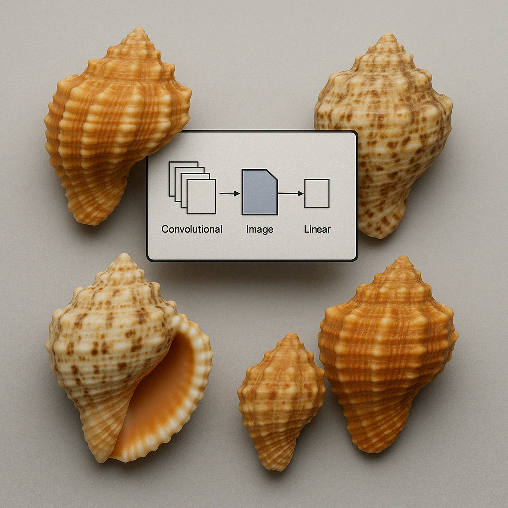
Embedder model
Image embeddings were generated using a convolutional neural network implemented in TensorFlow/Keras. The backbone architecture used in this study was EfficientNetV2B2, initialized with ImageNet pretrained weights [8, 10]. Although general-purpose foundation models such as CLIP and DINOv2 were considered (see Introduction), EfficientNetV2B2 was selected for three practical reasons: (i) it allowed domain-controlled VICReg training directly on the collector image pool, avoiding potential domain mismatch from text-supervised CLIP pretraining; (ii) it provided a fully reproducible training pipeline with fixed seeds, whereas large foundation-model inference can vary across library versions; and (iii) its moderate parameter count was compatible with the computational resources available for repeated bootstrap runs across the full candidate set. The original classification head was removed, and the backbone output was followed by global average pooling, a dense projection layer of 512 dimensions, and batch normalization to produce the final embedding vector. The backbone was kept frozen during training, and only the projection layers were optimized.
Training was performed using a dual-manifest setup, with separate manifests for the seed/training images and the inference images. The training manifest was used to optimize the embedder, whereas the inference manifest was used subsequently for embedding extraction and downstream geometric evaluation. All images were decoded as three-channel RGB images and resized to 384 × 384 pixels prior to input to the network.
The embedder was trained using the VICReg (Variance-Invariance-Covariance Regularization) objective, a self-supervised representation learning method that combines an invariance term, a variance regularization term, and a covariance regularization term [9]. The respective loss weights were 25.0, 25.0, and 1.0, with a variance regularization epsilon of 1 × 10⁻⁴. Embeddings were normalized only afterwards when cosine-distance-based analyses were performed.
Optimization was performed with the Adam optimizer using a learning rate of 1 × 10⁻⁴. Training was run for a maximum of 40 epochs and monitored using training loss. Early stopping was applied with a patience of four epochs and restoration of the best weights. In addition, the learning rate was reduced on plateau by a factor of 0.5 after two epochs without improvement, with a minimum learning rate of 1 × 10⁻⁶. The batch size was 32. Gradient accumulation with two accumulation steps was used in the VICReg trainer. Mixed-precision computation was enabled, and fixed random seeds were used for Python, NumPy, and TensorFlow to improve reproducibility.
After training, the embedder was exported as a standalone model for subsequent embedding extraction and species-level analyses.
Embedding extraction
The trained embedder described above was loaded as a standalone TensorFlow/Keras model and applied to the candidate manifest to generate image embeddings for downstream diagnostic analysis. The candidate manifest provided the image path and species label for each image, with optional metadata fields including source, island, background, and source-specific record identifier. Images were decoded as three-channel RGB images, resized to 384 × 384 pixels, and preprocessed using the EfficientNetV2 input transformation prior to inference.
Embeddings were generated in batches of 32 images and exported as floating-point feature vectors. For all neighborhood-based analyses, the embeddings were subsequently L2-normalized and cosine distance was used as the similarity metric. Nearest-neighbor analysis was performed with the NearestNeighbors implementation in scikit-learn [46]. For each image, the 25 nearest neighbors were retrieved in embedding space, excluding the image itself from the neighborhood.
Several per-image diagnostic variables were then calculated. Let ksame denote the number of same-species images among the 25 nearest neighbors. The same-species neighbor fraction was defined as ksame/25, and the different-species neighbor fraction as its complement. The nearest same-species distance and nearest different-species distance were obtained as the minimum cosine distance to any same-species and different-species neighbor, respectively, within the retrieved neighborhood. A margin statistic was calculated as the nearest different-species distance minus the nearest same-species distance, such that positive values indicate that the closest conspecific image is nearer than the closest heterospecific image. Neighborhood label entropy was also computed to quantify the degree of local class mixing in embedding space.
In addition, a per-image suspicion score was calculated to prioritize potentially problematic records for review. This score combined neighborhood disagreement and cross-species proximity according to: suspicion = (1 − kNN same fraction) × (1 − clipped nearest different-species distance). Higher values therefore indicate images whose local neighborhood contains relatively few conspecifics and whose nearest heterospecific neighbor lies close in embedding space.
To quantify iteration-to-iteration stability, intra-species neighbor sets were computed using the 10 nearest conspecific neighbors for each image. When a previous iteration was available, the overlap between current and previous within-species neighbor sets was measured using the Jaccard index. Species-level neighborhood stability was summarized as the mean intra-species Jaccard similarity and its standard deviation across images. In addition, for each species, the 50 highest-suspicion images were retained as a review queue, and the Jaccard similarity of this queue between successive iterations was calculated as an additional stability measure.
Potential within-species substructure was assessed using DBSCAN clustering in the normalized embedding space with cosine distance, using an epsilon value of 0.12 and a minimum of 5 samples per cluster [11]. Clusters with fewer than 10 images were not considered major clusters. A species was marked as a potential split candidate when at least two major clusters were detected and these clusters could not be explained primarily by nuisance variables such as image source or background. To evaluate such nuisance effects, cluster purity was calculated for available nuisance metadata fields, and the maximum purity across major clusters was retained.
Species-level embedding diagnostics
Species-level diagnostic metrics were calculated in embedding space to summarize within-species compactness, neighborhood purity, outlier burden, and structural stability. These metrics were computed on the deduplicated seed/reference set used as the trusted comparison pool for neighbor-based statistics. Deduplication retained only the primary assignment for each unique image, defined as the lowest row_idx for each image identity, and manually excluded images were removed prior to analysis. Neighbor-based statistics were calculated relative to the seed list only, such that candidate images were not allowed to support one another. This reduced circular reinforcement by noisy candidates and limited cluster drift.
Cosine distance was used to quantify similarity in embedding space. For each image, let dsame denote the cosine distance to the nearest image of the same species and ddiff the cosine distance to the nearest image of any different species. Let ksame denote the number of same-species neighbors among the top-K nearest neighbors, with K = 25 for the neighborhood-purity calculations. At image level, cohesion was defined as ksame/K, margin as ddiff − dsame, and stability as 1 − σ, where σ is the raw suspicion score produced by the model. Metric orientation was standardized such that higher values indicate better performance. The choice 𝐾=25 was adopted as a fixed benchmark setting to provide consistent local-purity estimates across species while avoiding the excessive variance associated with very small neighborhoods. Accordingly, it should be regarded as a heuristic operational parameter, and the main biological interpretation relies more on relative species ranking and recurrent patterns than on the exact value of 𝐾 in isolation.
The number of images for a species was defined as the number of analyzed seed images remaining after deduplication and exclusion filtering. Species-level cohesion was calculated as the mean of the per-image same-species neighbor fraction. This metric represents the average proportion of nearest neighbors belonging to the focal species and therefore quantifies local manifold density and label consistency. Neighborhood purity was quantified as the mean fraction of same-species neighbors among the 25 nearest neighbors of each image, using the seed/reference set as the search space.
Outlier rate was defined as the proportion of images failing a local-support rule. In the main species analysis, an image was flagged as an outlier when its local same-species neighbor fraction was below 0.40. The species-level outlier rate was then calculated as the percentage of images classified as outliers within that species. Elevated outlier rates were interpreted as evidence of heterogeneous species structure, possible label noise, or species bins containing multiple concepts.
Species-level stability was computed as a neighborhood-reproducibility measure, reported as mean Jaccard similarity. This metric quantifies how consistently the same nearest neighbors are recovered across embedder iterations; higher values indicate a more stable species manifold and more reproducible local structure across runs. Within the same framework, the per-image stability diagnostic was defined as 1 − σ, whereas the aggregated species-level stability statistic corresponded to mean Jaccard neighborhood stability.
Global Inference Mapping of Species Relationships
To quantify boundary mixing among candidate species in the embedding space, a global inference map in the form of a pairwise interference matrix was constructed. Each matrix cell represents the directional degree of confusion from a source species A toward a rival species B. This map was designed to provide a global overview of how well the trusted reference set partitions morphological variation and to identify species pairs showing potential taxonomic overlap, ambiguous boundaries, or insufficient separation.
The matrix was computed from image embeddings derived from the representation model used in the Seed & Grow workflow. Pairwise interference was summarized with a Pair Confusion Score (PCS), defined as a weighted ensemble of three complementary components: local neighborhood mixing, geometric margin confusion, and statistical tail separation. In the default implementation, the PCS between species A and B was calculated as:
with default weights \( w_1 = 0.5 \), \( w_2 = 0.3 \), and \( w_3 = 0.2 \). Distances in embedding space were computed using cosine distance \( (1 - \cos \theta) \).
The first component, neighborhood support (\( C_{knn} \)), measures local mixing between species. For each image belonging to source species A, the proportion of its \( K \) nearest neighbors that belonged to rival species B was calculated, and these proportions were averaged across all images in A. In the reference methodology, the neighborhood size was typically set to \( K = 25 \). High \( C_{knn} \) values indicate that specimens of species A are locally surrounded by specimens assigned to species B.
The second component, geometric margin confusion (\( C_{margin} \)), quantifies overlap relative to species prototypes or medoids. For each image in species A, the distance to its own closest medoid was compared with the distance to the closest medoid of rival species B. Confusion increased when a specimen was closer to the rival medoid than to its own, or when the margin between these two distances was small. This component was intended to capture boundary-level ambiguity and prototype overlap in the embedding manifold.
The third component, statistical tail separation (\( C_{tail} \)), evaluates whether the inter-species gap is sufficiently larger than the within-species spread. Specifically, the 5th percentile of cross-species distances between A and B was compared with the median within-species distance of the two species. Confusion was increased when the inter-species gap was small relative to the internal spread, indicating limited separation between the tails of the two populations.
Because the score is directional, \( PCS(A,B) \) is not necessarily equal to \( PCS(B,A) \). This directional formulation is useful in cases where one species shows a stronger tendency to overlap into the representation space of another species than vice versa. After computing all pairwise PCS values, the results were arranged into a square species-by-species matrix and visualized as a heatmap, here termed the global inference map. Darker or near-zero values indicate little detectable interference, whereas higher values indicate stronger pairwise confusion.
Following the methodological interpretation framework, PCS values above \( 0.40 \) were considered indicative of critical ambiguity, values between \( 0.15 \) and \( 0.40 \) as moderate boundary friction, and values below \( 0.15 \) as low interference, corresponding to relatively clean separation. These thresholds were used as practical diagnostic ranges to prioritize species pairs for expert review, seed hardening, or targeted expansion of the trusted reference set.
The global inference map was used as a diagnostic layer within the broader delimitation workflow. Rather than serving as an autonomous taxonomic decision rule, it was used to identify species pairs requiring closer inspection, especially where morphological similarity, sparse sampling, mislabeled seeds, or incomplete coverage of intraspecific variation might lead to artificial mixing in the embedding space.
Bootstrap-based stability analysis and uncertainty quantification
To quantify the robustness of embedding-based species delimitation results, a bootstrap resampling framework designed to measure both within-species cohesion and between-species interference stability under repeated perturbation of the reference data. This analysis was introduced as a core benchmark component because point estimates alone are insufficient for defensible taxonomic triage: species delimitation decisions should remain interpretable under modest variation in the sampled evidence. The bootstrap analysis therefore served as a non-parametric uncertainty assessment for ranking stability, outlier persistence, and pairwise interference patterns. The underlying framework distinguishes two complementary levels of analysis: Level 1, which evaluates internal cluster geometry, and Level 2, which evaluates robustness of class assignments under perturbation of the seed/reference set.
All calculations were performed in embedding space using cosine distance / cosine similarity, consistent with the project bootstrap workflow. For each target run, repeated bootstrap replicates were generated by sampling with replacement from the available images of each focal species. In the analyses reported here, the number of replicates was set to B = 500, as shown in the stability result panels. The resulting replicate distributions were summarized using means, standard deviations, confidence intervals, rank persistence measures, and flag frequencies. Calculations were implemented in the project bootstrap pipeline using cosine-distance embeddings.
The main contribution of this component is not another static performance score, but the introduction of stability and uncertainty as explicit criteria for AI-assisted taxonomic triage. This makes the workflow more reproducible and defensible, especially in settings where marginal classification improvements have plateaued.
Level 1: geometric cohesion of species clusters
Level 1 bootstrap analysis was used to characterize the geometric density of each species cluster. In this context, geometric density represents the mean cosine similarity between the images assigned to a species and the medoid of that species within each bootstrap replicate. This measure evaluates how well the medoid represents the central tendency of the cluster and therefore provides a measure of internal morphological compactness in embedding space. High values indicate a tight and coherent cluster, whereas low values indicate a diffuse or fragmented concept that may reflect broad intraspecific variation, image noise, unresolved multimodality, or mixed bins.
Formally, for species C, bootstrap replicate b, resampled image set Cb, and medoid mC,b, geometric density was computed as:
B ∑b=1B ( 1
|Cb| ∑x ∈ Cb (1 - distcos(x, mC,b)) )
Thus, Level 1 measures the average similarity of class members to the bootstrap-derived medoid across replicates. For each species, the Level 1 analysis produced a distribution of cohesion values from which the mean cohesion, standard deviation, and cohesion confidence interval were derived. In addition, worst-rank frequency was recorded to quantify how often a species remained among the least cohesive clusters across replicates.
Outlier behavior was also tracked within the same resampling framework. Images identified as outliers within individual replicates were monitored across the full bootstrap series. This yielded two uncertainty-aware outputs: an outlier confidence interval and a flag frequency, defined as the percentage of bootstrap replicates in which a given image or species-level outlier condition remained flagged. Persistent flags were interpreted as stronger evidence of reproducible instability than outlier calls that appeared only sporadically.
Level 2: bootstrap stability of taxonomic assignments
Level 2 bootstrap analysis was used to measure taxonomic boundary robustness. Unlike Level 1, which focuses on internal cluster compactness, Level 2 evaluates how stable the species assignment structure remains when the reference seed sets are perturbed by resampling. In the project methodology, stability is defined as the retention rate of original class assignments after recalculating provisional medoids from randomized subsamples. Low stability indicates sensitivity to the exact composition of the seed set and therefore suggests concept overlap, weak morphological separation, or dependence on a limited number of exemplar images.
If Lorig(x) denotes the original species label of image x, and Lb(x) the label assigned to that image in bootstrap replicate b, then species-level stability for class C was computed as:
B ∑b=1B ( 1
|C| ∑x ∈ C 𝟙[Lb(x) = Lorig(x)] )
For each species, the Level 2 analysis yielded a bootstrap distribution of retention scores. From this distribution the mean stability, standard deviation, and a stability confidence interval is calculated. Species with persistently low stability or high worst-rank frequency were interpreted as taxonomically fragile under perturbation of the seed set.
Pairwise interference stability and Top-10 persistence
In addition to species-level summaries, pairwise interference stability was evaluated. For each bootstrap replicate, the workflow recorded the extent to which particular species pairs shared local neighborhood structure in embedding space. This was summarized as a pairwise k-nearest-neighbor share statistic and tracked across replicates. For each species pair, the replicate distribution was summarized by its mean, standard deviation, and confidence interval.
To make these interference patterns interpretable at the comparative level, Top-10 persistence was also computed, defined as the percentage of bootstrap replicates in which a given species pair remained among the ten strongest interference pairs. This measure distinguishes persistent boundary problems from pairs that appear only intermittently. A pair with high average interference but low Top-10 persistence was interpreted as unstable or context-dependent, whereas a pair with both high interference and high persistence was interpreted as a reproducible candidate for manual taxonomic review.
Confidence intervals and ranking stability
Confidence intervals were used throughout to quantify uncertainty around bootstrap-derived means. For cohesion, outlier burden, and pairwise interference metrics, the interval estimates summarize how strongly the measured value depends on the particular resampled composition of the data. However, because triage decisions are often rank-based rather than threshold-based, central tendency alone is not sufficient. For this reason, the workflow also recorded flag frequency and Top-10 persistence as ranking-stability measures. These outputs identify whether a species, image, or pair remains problematic across repeated perturbations, rather than only in the original run.
Role in the species-delimitation workflow
The bootstrap stability analysis was incorporated as an uncertainty-aware layer on top of the embedding-based species delimitation workflow. The two bootstrap levels were used for distinct but complementary purposes. Level 1 was used to assess internal morphological uniformity and to detect scattered or potentially mixed species concepts. Level 2 was used to test whether observed taxonomic boundaries remained stable when the underlying seed evidence was perturbed. A species could therefore show a compact internal geometry while still displaying unstable taxonomic boundaries under seed resampling, or vice versa. This separation of geometric cohesion from assignment robustness is central to the interpretation of the resulting stability plots.
Overall, this stability framework provides a reproducible basis for prioritizing species, outliers, and interfering species pairs for expert review. In this sense, the benchmark contribution is not simply improved discrimination, but improved defensibility: the ability to show that problematic clusters and rival pairs remain problematic under repeated perturbation of the available evidence.
Illustrative output panels
The bootstrap workflow produces result panels at both levels. The Level 1 panel reports species cluster density summaries and pairwise interference rankings based on geometric cohesion, whereas the Level 2 panel reports species bootstrap stability and pairwise interference rankings under seed perturbation.
Sequence filtering, alignment, and accepted-species grouping
An aligned FASTA file containing the retained COX1 sequences was used as the molecular input for distance analysis. Sequence matching between the FASTA file and the metadata table was based on accession name.
All downstream summaries were conducted at two levels. First, pairwise distances were computed at the accession level, preserving all retained sequences. Second, accession-level results were summarized by accepted species name. This two-stage design avoided premature collapsing of within-species variation while allowing synonymized labels and reassigned nominal taxa to be treated as a single accepted taxon in the biological summaries.
Sequence coverage was uneven among accepted species. Accordingly, all retained accessions were used for interspecific comparisons, but within-species summaries were interpreted in relation to sample size. Species represented by a single sequence were retained for between-species distance analyses but did not contribute to within-species dispersion estimates. Species represented by two sequences were treated as descriptive only, whereas more stable within-species summaries were derived preferentially from species represented by three or more sequences.
Pairwise genetic distance analysis
Pairwise mitochondrial distances were computed from the aligned COX1 sequences at the accession level. The primary metric used was uncorrected p-distance, defined as the proportion of differing nucleotide sites among compared sites for each sequence pair. Only positions containing valid unambiguous nucleotides (A, C, G, or T) in both sequences were included in a comparison. Positions containing gaps or ambiguous symbols were excluded on a pairwise basis. Comparisons with fewer than a minimum number of valid aligned sites were discarded. The accession-level results were stored both as a square distance matrix and as a long-format pairwise table containing the two accession identifiers, their accepted species assignments, the pairwise distance, the number of compared sites, and an indicator of whether the two sequences belonged to the same accepted species.
From the accession-level table, species-level molecular summaries were derived. For each accepted species, within-species statistics included the number of sequences, number of within-species accession pairs, mean within-species p-distance, median within-species p-distance, minimum within-species distance, and maximum within-species distance. For each accepted species pair, between-species statistics included the number of contributing accession pairs, mean interspecific p-distance, median interspecific p-distance, minimum interspecific distance, and maximum interspecific distance; the full minimum interspecific COX1 distance matrix is provided in Supplementary Table 10. In addition, for each accepted species, the nearest other species was identified as the species with the smallest observed minimum interspecific distance.
As a sensitivity option, Kimura 2-parameter (K2P) distances could also be computed from the same alignment, but the primary workflow used p-distance because of its transparency and direct interpretability for the comparative analyses presented here.
Integration with embedding-based diagnostics
The mitochondrial analyses were designed as an orthogonal validation layer for the image-embedding workflow rather than as an automatic species-delimitation rule. Molecular summaries were therefore compared with diagnostics generated from the image-embedding analyses. Two types of integration were performed.
First, species-level molecular summaries were merged with species-level embedder diagnostics, including the number of images, same-class neighborhood purity, outlier rate, cross-source nearest-neighbor rate, major-cluster count, and split-candidate status. Because embedder outputs occasionally used project-level or morphotype-style labels rather than accepted species names, embedder labels were normalized before merging. Parenthetical qualifiers and variant labels, such as color-based morphotype annotations, were collapsed to their corresponding accepted species assignment. When multiple embedder labels mapped to the same accepted species, their statistics were aggregated at the accepted-species level prior to integration.
Second, pairwise molecular summaries were merged with cross-class embedding diagnostics derived from nearest inter-class image pairs. Image-level cross-class pairs were first normalized to accepted species names and then collapsed to species-pair summaries. For each species pair, the embedding analysis yielded the number of contributing cross-class image pairs and summary statistics for cross-class embedding distance, including the minimum, mean, and median nearest different-class distance. These species-pair embedding summaries were then joined to the corresponding mitochondrial species-pair table to assess whether strong image-space confusion tended to coincide with low interspecific COX1 distance.
Comparative visualization and interpretation
Three classes of comparative visualizations were generated from the merged molecular and embedding tables. First, within-species mean COX1 distance was plotted against the embedding-derived outlier rate to examine whether image-space heterogeneity tracked mitochondrial spread. Second, the minimum COX1 distance to the nearest other species was plotted against same-class neighborhood purity to test whether genetically well-separated taxa also showed stronger embedding separation. Third, interspecific COX1 distance was plotted against cross-class embedding proximity for species pairs represented in both data layers. These plots were used for comparative interpretation rather than as formal delimitation criteria.
In this framework, concordance between embedding proximity and mitochondrial proximity was interpreted as support that image-space structure, within the represented taxa, could reflect biologically meaningful relatedness Conversely, strong embedding confusion combined with relatively large mitochondrial separation was interpreted as suggestive of image-driven or label-driven ambiguity. Discordant cases were not treated as automatic evidence for taxonomic revision, because mitochondrial data represent a single inherited genome and may disagree with species boundaries for several evolutionary reasons. Molecular evidence was therefore used here as an external plausibility signal in aggregate, while final curation and taxonomic interpretation remained human-led.
Results
Species Delimitation Workflow
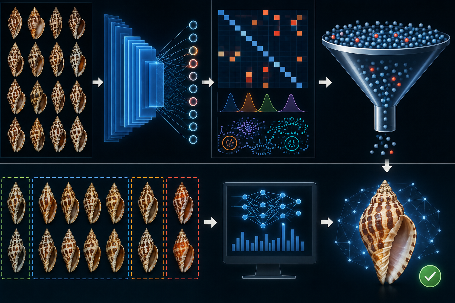
In this study, species delimitation is supported by a human-led, embedding-assisted iterative curation workflow (“Seed & Grow”). The goal of this workflow is not to let the model make taxonomic decisions, but to use embedding-derived diagnostics to prioritize human review and to progressively improve the quality and consistency of the species image dataset. Starting from an initial curated subset (“seed”), a model is trained to generate embeddings for a broader candidate pool. Quantitative diagnostics (e.g., neighborhood structure, boundary ambiguity, and cluster behavior) are then used to identify high-value images and clusters for expert inspection. Based on this evidence, the human reviewer makes the final curation decisions (e.g., acceptance, removal, or merge/split evaluation), after which the curated set is updated and the cycle is repeated. This iterative design separates taxonomic judgment (human) from triage and prioritization (model-assisted), while providing a reproducible framework for systematic dataset refinement.
A key design choice of this workflow is that not all available images are used directly for training at each iteration. In heterogeneous collector imagery, labels may be inconsistent, uncertain, or historically assigned under different taxonomic concepts, and image quality/viewpoint variation can be substantial. Training on the full image pool without curation would propagate label noise into the embedding space, potentially obscuring biologically meaningful structure and reducing the value of embedding-derived diagnostics for human review. The Seed & Grow strategy therefore begins from a curated subset and expands iteratively, allowing human validation to control error propagation while progressively increasing dataset coverage.
This is particularly important in a species-delimitation context, where the objective is not only classification performance but also reliable identification of ambiguity, conflict, and potential over-lumping/over-splitting. If all images are treated as equally trustworthy training labels from the outset, the model may learn to reproduce existing labeling inconsistencies rather than expose them. By separating a curated training set from a broader candidate pool, the workflow preserves a stable reference signal while using embeddings to triage which images and clusters should be reviewed next.
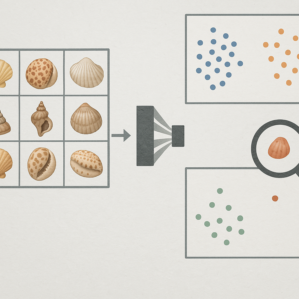
Figure 1. The Seed & Grow Iterative Curation Workflow
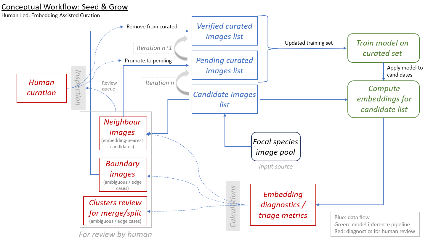
Figure 1: The Seed & Grow Iterative Curation Workflow Overview of a human-led, embedding-assisted
workflow for iterative
species-dataset discovery and curation. A curated set is used to train/update a model, which computes
embeddings for candidate images.
Embedding-derived diagnostics prioritize high-value review targets (e.g., neighbours, boundary cases, and
cluster structure), after
which expert human decisions update the curated dataset for the next iteration.
- Blue Boxes (Data Entities): Represent the evolving states of the image dataset. This ranges from the source image pool (start of the workflow) over candidate image pool to "Verified" (gold-standard) and "Pending" (finally accepted by human review; queued for inclusion in the next training iteration - not yet consumed by the current model run) curated sets. Green Boxes (Inference Pipeline): Denote the automated computational stages, including neural network training on curated "seeds" and the subsequent generation of high-dimensional embeddings for the candidate pool. Red Boxes (Triage & Diagnostics): Highlight the active learning outputs — statistical metrics (e.g., entropy, k-NN agreement) and categorized lists designed to focus human effort on ambiguous or high-impact data points. Solid Arrows (Data Flow): Indicate the primary directional movement of data and model weights through the automated pipeline. Dashed Arrows (Expert Decisions and triage metrics): Represent the "Human-in-the-loop" interactions, where expert decisions (promotion, removal, or taxonomic revision) modify the state of the dataset based on diagnostic evidence. Grey Vertical Bars (Interface Gates): Mark the transition points where raw Calculations are transformed into actionable Inspection tasks for the user and human decisions made on visual inspection and metrics.
- 2. Process Stages: Focal Species Image Pool: The primary input source of unclassified or unaligned specimens available for discovery. Iteration Loop (n -> n+1): The core recursive mechanic of the workflow. Human-validated candidates are promoted to the curated set, which then serves as the "seed" for the subsequent iteration's model training, progressively refining the model's discriminatory power. Embedding Diagnostics: The calculation of triage metrics that identify Neighbour images (candidates similar to known seeds) and Boundary images (cases of high ambiguity or class interference). Clusters Review (Merge/Split): A critical taxonomic decision gate where the expert evaluates whether the current embedding space suggests the need to merge existing species labels or split a single class into multiple distinct taxa. Human Curation: The final expert-led validation stage that ensures taxonomic integrity and data quality, transforming model-assisted suggestions into a high quality dataset.
In the workflow, the curated dataset is represented as two operational states: Verified and Pending. Verified images are final human-accepted examples that have already been incorporated into the current curated training set. Pending images are also final human-accepted examples, but are queued for inclusion in the next training iteration (i.e., accepted but not yet consumed by the current model run). This separation distinguishes curation finality from pipeline timing.
Embedding-derived diagnostics are used to prioritize expert attention, not to automate taxonomic decisions. In particular, neighbour and boundary review queues are intended to accelerate identification of likely additions, ambiguous cases, and potential labeling inconsistencies, while cluster review supports human assessment of possible over-lumping or over-splitting. Final decisions on acceptance, removal, or taxonomic interpretation remain human-led.
A typical iteration begins by updating the curated lists based on the previous review round. The model is then trained or updated on the curated set, embeddings are computed for candidate images, and triage metrics are calculated to generate prioritized review targets. After expert inspection, accepted images are added to the pending curated state (for the next training iteration), while removals or reassignments update the candidate/curated pools accordingly. The cycle is then repeated, progressively improving coverage and consistency of the dataset.
Species-level embedding diagnostics
Species-level embedding quality varied markedly among the examined Conus taxa and morphotypes. Several taxa showed highly coherent and stable embedding structure, whereas others displayed weak local cohesion, high outlier rates, and low neighborhood stability, indicating heterogeneous image sets or poor separation in embedding space.
Table 2. Species-level embedding quality metrics
| Species/Morphotype | # images | Cohesion | kNN same (@25) | Outliers % | Stability |
|---|---|---|---|---|---|
| C. calhetae | 24 | 0.10 | 0.11 | 100% | 0.24 |
| C. ermineus | 129 | 0.97 | 0.97 | 0% | 0.97 |
| C. galeao | 51 | 0.22 | 0.21 | 90% | 0.30 |
| C. genuanus | 169 | 1.00 | 0.99 | 0% | 1.00 |
| C. gonsaloi | 29 | 0.20 | 0.19 | 90% | 0.29 |
| C. infinitus | 90 | 0.50 | 0.60 | 22% | 0.54 |
| C. isabelarum | 29 | 0.10 | 0.11 | 100% | 0.25 |
| C. maioensis | 138 | 0.93 | 0.93 | 6% | 0.94 |
| C. perrineae | 46 | 0.75 | 0.96 | 0% | 0.76 |
| C. perrineae (brown) | 27 | 0.32 | 0.48 | 33% | 0.34 |
| C. raulsilvai | 24 | 0.19 | 0.28 | 67% | 0.22 |
| C. trochulus | 59 | 0.72 | 0.74 | 12% | 0.75 |
| C. venulatus | 110 | 0.92 | 0.92 | 7% | 0.93 |
Table 2: Reported metrics include the number of analyzed images, cohesion, kNN same (@25), outlier percentage, and stability. Higher cohesion, neighborhood purity, and stability values indicate stronger within-group consistency in embedding space, whereas lower outlier percentages indicate more homogeneous image sets. C. perrineae (brown) denotes a workflow-defined morphotype rather than a formally recognized species; it was evaluated using the same candidate pool as C. perrineae, but with seeds restricted to the brown variant.
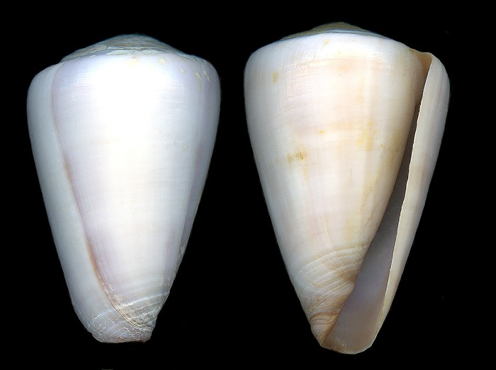
The strongest performance was observed for C. genuanus, which showed near-perfect values across all metrics (cohesion 1.00, kNN same @25 = 0.99, outliers 0%, stability 1.00). Similarly, C. ermineus, C. maioensis, and C. venulatus showed consistently high cohesion (0.92–0.97), high neighborhood purity (0.92–0.97), low outlier rates (0–7%), and high stability (0.93–0.97), indicating compact and reproducible species structure in embedding space. C. perrineae and C. trochulus also performed well overall, although with somewhat lower cohesion and stability values than the strongest group.
Intermediate performance was observed for C. infinitus and the morphotype C. perrineae (brown). C. infinitus showed moderate cohesion (0.50), moderate neighborhood purity (0.60), an outlier rate of 22%, and stability of 0.54, suggesting only partial internal consistency. The brown morphotype of C. perrineae showed even lower cohesion (0.32) and stability (0.34), together with an elevated outlier rate (33%), indicating weaker embedding compactness than the nominal form.
In contrast, several taxa showed poor embedding quality. C. calhetae, C. galeao, C. gonsaloi, C. isabelarum, and C. raulsilvai all had low cohesion (0.10–0.22), low kNN same values (0.11–0.28), high outlier rates (67–100%), and low stability (0.22–0.30). These taxa therefore lacked a compact and reproducible neighborhood structure in the learned embedding space. Among these, C. calhetae and C. isabelarum were the weakest cases, with 100% outliers and very low cohesion and stability values.
Overall, the results indicate that the embedding model captured strong and consistent structure for some species, while others remained poorly resolved. High-performing taxa were characterized by simultaneously high cohesion, high local neighborhood purity, low outlier burden, and high iteration-to-iteration stability, whereas low-performing taxa showed the opposite pattern. This heterogeneity suggests that embedding quality is species-dependent and that some taxa or morphotypes may require additional review, improved image curation, or alternative delimitation strategies.
Lower performance in some taxa may partly reflect limited image availability, as small sample sizes can reduce the stability and representativeness of local neighborhood structure in embedding space. However, sample size alone does not fully explain the observed variation, because taxa with comparable numbers of images differed substantially in cohesion, neighborhood purity, outlier rate, and stability.
Global Inference Mapping of Species Relationships
The global inference map showed that most species pairs had low to moderate directional interference, with only a limited number of pairwise comparisons reaching higher Pair Confusion Score (PCS) values. Within the analyzed dataset and under the current assignment structure, interference was therefore concentrated in a restricted subset of species pairs rather than being broadly distributed across the full matrix. This pattern should be interpreted as a property of the present embedding representation and label structure, not as definitive evidence of taxonomic separation.
Figure 2. Global inference map showing directional pairwise interference among analyzed species groups
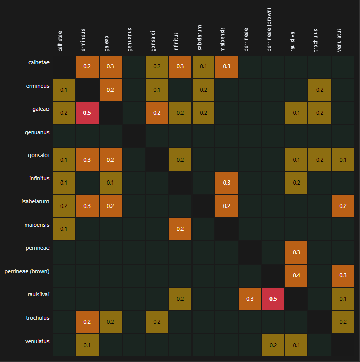
The strongest directional interference signals were observed for raulsilvai → perrineae (brown) and galeao → ermineus, both with a PCS of 0.46. These were the highest values in the ranked interference table and represent the most pronounced pairwise ambiguities detected by the current analysis. In the case of galeao → ermineus, the corresponding kNN value was also high (0.49), indicating strong local neighborhood mixing. By contrast, raulsilvai → perrineae (brown) combined a similarly high PCS with a more moderate kNN value (0.29), suggesting that its elevated score was not driven solely by nearest-neighbor overlap, but likely also by margin-based and tail-based proximity.
A particularly notable pattern involved the relationship between raulsilvai and perrineae (brown). The interference score was high in both directions, with raulsilvai → perrineae (brown) at 0.46 and the reverse direction, perrineae (brown) → raulsilvai, at 0.38. This bidirectional pattern indicates that these two groups occupy weakly separated regions in the current embedding space. The asymmetry between both directions nevertheless suggests that the overlap is not balanced, with raulsilvai appearing to intrude more strongly into the region associated with perrineae (brown) than the reverse. A related but weaker signal was also observed for perrineae → raulsilvai (PCS = 0.28), indicating that interference around raulsilvai may extend beyond the brown form alone and may involve the broader perrineae complex.
Several additional directional pairs showed moderate interference. These included isabelarum → ermineus (PCS = 0.34, kNN = 0.34), calhetae → infinitus (0.31), perrineae (brown) → venulatus (0.30, kNN = 0.30), and gonsaloi → ermineus (0.29). Other pairs in the same range included calhetae → maioensis (0.27), calhetae → galeao (0.26), infinitus → maioensis (0.26), raulsilvai → perrineae (0.26), gonsaloi → galeao (0.25), isabelarum → venulatus (0.25), and isabelarum → maioensis (0.24). These results suggest that the main interference structure was not diffuse across all species, but instead concentrated in a relatively small number of directional relationships.
The map also showed clear evidence of directionality, consistent with the non-symmetric definition of PCS. For example, galeao → ermineus reached 0.46, whereas the reverse direction, ermineus → galeao, was lower at 0.24. This asymmetry indicates that images assigned to galeao more frequently occupy neighborhoods or margins associated with ermineus than the reverse. Similar directional imbalances were visible elsewhere in the ranked list and indicate that the global inference map captures more than undirected similarity: it reflects how strongly one group projects into the representational space of another under the current model and assignments.
At the matrix level, the interference structure appeared sparse rather than broadly diffuse. Most cells in the heatmap remained dark or near-zero, while elevated scores were concentrated in a limited subset of species pairs. Under the present analytical framework, this indicates that the model does not show generalized pairwise interference across all groups, but instead highlights localized zones of overlap or boundary weakness. These localized signals are especially relevant for prioritizing expert review, because they allow attention to be focused on a manageable set of potentially problematic species pairs.
Taken together, the global inference map functioned as an effective screening and prioritization layer within the broader delimitation workflow. The most prominent interference patterns involved the pairs raulsilvai–perrineae (brown) and galeao–ermineus, with additional moderate signals involving isabelarum, calhetae, infinitus, maioensis, and venulatus. These pairs represent the highest-priority candidates for deeper specimen-level inspection, reassessment of seed list quality or assignment quality, and possible expansion of reference coverage to better capture within-group variation.
Bootstrap stability analysis identifies both persistent weak species clusters and reproducible interference pairs
Bootstrap-based stability analysis revealed marked heterogeneity among species with respect to both internal geometric cohesion (Level 1) and assignment robustness under seed perturbation (Level 2). The outputs also showed that several pairwise interference relationships were not isolated events, but recurred across bootstrap replicates with substantial Top-10 persistence. Taken together, these results indicate that the workflow captures not only point estimates of embedding structure, but also the uncertainty and rank stability of candidate taxonomic problem cases. Metric definitions for geometric density and bootstrap stability follow the underlying bootstrap framework.
In the Level 1 analysis, species differed strongly in geometric density, indicating variation in how compactly each species formed a cluster around its medoid in embedding space (Table 3). Several species showed comparatively low density and extremely high worst-rank frequency, meaning that they repeatedly ranked among the weakest clusters across bootstrap replicates. The lowest-density species were galeao (0.4677 ± 0.0283), isabelarum (0.4504 ± 0.0455), and calhetae (0.5530 ± 0.0531), all with worst-rank frequencies close to or equal to 100% (Table 3). By contrast, species such as genuanus (0.9694 ± 0.0027), perrineae (brown) (0.9584 ± 0.0060), and perrineae (0.9476 ± 0.0028) appeared highly cohesive and did not recur among the lowest-ranked clusters in the the Level 1 bootstrap results (Table 3).
Table 3. Species cluster density Level 1 panel
| Species | Geometric Density (Mean ± SD) | Worst-Rank Frequency |
|---|---|---|
| galeao | 0.4677 ± 0.0283 | 100.0% |
| isabelarum | 0.4504 ± 0.0455 | 100.0% |
| calhetae | 0.5530 ± 0.0531 | 99.6% |
| ermineus | 0.6461 ± 0.0077 | 98.6% |
| trochulus | 0.6524 ± 0.0133 | 93.8% |
| gonsaloi | 0.6982 ± 0.0294 | 8.0% |
| perrineae (brown) | 0.9584 ± 0.0060 | 0.0% |
| perrineae | 0.9476 ± 0.0028 | 0.0% |
| infinitus | 0.8259 ± 0.0095 | 0.0% |
| maioensis | 0.7383 ± 0.0093 | 0.0% |
| raulsilvai | 0.9098 ± 0.0107 | 0.0% |
| venulatus | 0.8093 ± 0.0123 | 0.0% |
| genuanus | 0.9694 ± 0.0027 | 0.0% |
Table 3. Species cluster density Level 1. Bootstrap summary of species-level geometric density in embedding space for the Level 1 analysis. Geometric density is reported as mean ± SD across bootstrap replicates and summarizes how compactly each species forms a cluster around its medoid in the learned embedding space. Worst-rank frequency indicates how often a species appeared among the weakest clusters across replicates; higher values therefore indicate persistently low cohesion and reduced structural robustness.
The Level 1 pairwise interference results showed that some species pairs repeatedly shared local neighborhood structure (Table 4). The strongest visible interference signal was observed for calhetae × galeao (kNN share 0.2656 ± 0.0867; Top-10 frequency 68.2%), followed by galeao × gonsaloi (0.2672 ± 0.1037; 65.4%). Additional high-ranking pairs involved galeao with several other taxa, including perrineae, trochulus, and raulsilvai, suggesting that galeao occupies a locally unstable position in the embedding space represented by this run (Table 4).
The Level 1 pattern suggests that some species are internally diffuse and repeatedly rank among the least cohesive clusters, while a limited set of species pairs recur as strong interference candidates. This combination is consistent with the intended use of Level 1 as a screen for geometrically weak or potentially mixed concepts.
Table 4. Pairwise interference Level 1.
| Species Pair | kNN Share (Mean ± SD) | Top-10 Frequency |
|---|---|---|
| calhetae × galeao | 0.2656 ± 0.0867 | 68.2% |
| galeao × gonsaloi | 0.2672 ± 0.1037 | 65.4% |
| galeao × perrineae | 0.1601 ± 0.1629 | 48.8% |
| galeao × trochulus | 0.1938 ± 0.1295 | 45.8% |
| gonsaloi × trochulus | 0.2109 ± 0.0784 | 45.6% |
| galeao × raulsilvai | 0.1464 ± 0.1499 | 45.2% |
| ermineus × isabelarum | 0.2297 ± 0.1102 | 43.8% |
| perrineae × trochulus | 0.1268 ± 0.1281 | 43.4% |
| ermineus × galeao | 0.2479 ± 0.1181 | 42.8% |
| perrineae (brown) × raulsilvai | 0.2021 ± 0.1543 | 39.6% |
| isabelarum × venulatus | 0.1525 ± 0.1165 | 33.2% |
| galeao × infinitus | 0.1315 ± 0.1353 | 32.6% |
| galeao × perrineae (brown) | 0.1279 ± 0.1321 | 32.0% |
| perrineae (brown) × trochulus | 0.1091 ± 0.1108 | 29.2% |
| calhetae × infinitus | 0.1518 ± 0.1255 | 27.0% |
| raulsilvai × trochulus | 0.1209 ± 0.1224 | 26.4% |
| isabelarum × maioensis | 0.1552 ± 0.0952 | 25.4% |
| gonsaloi × perrineae | 0.1036 ± 0.1177 | 24.0% |
| isabelarum × perrineae (brown) | 0.1007 ± 0.1156 | 23.0% |
Table 4. Pairwise interference Level 1. Bootstrap summary of recurrent species-pair interference in embedding space for the Level 1 analysis. kNN share is reported as mean ± SD across bootstrap replicates and quantifies the extent to which images from one species repeatedly share local neighborhood structure with another species. Top-10 frequency indicates how often a given pair ranked among the strongest interference pairs across replicates; higher values therefore indicate more persistent pairwise ambiguity.
The Level 2 analysis showed that species also differed strongly in bootstrap retention stability, that is, the extent to which original species assignments were preserved when the seed/reference set was resampled (Table 5). Several species displayed low stability together with very high worst-rank frequency. The least stable species were galeao (0.2166 ± 0.0802), isabelarum (0.2435 ± 0.0668), trochulus (0.2794 ± 0.0137), and calhetae (0.3036 ± 0.0477), all ranking near the bottom in almost all replicates (Table 5). By contrast, genuanus showed extremely high stability (0.9925 ± 0.0042), while perrineae (brown) (0.8948 ± 0.0734) and perrineae (0.8268 ± 0.0299) also appeared comparatively robust.
Table 5. Species bootstrap stability Level 2 panel
| Species | Bootstrap Stability (Mean ± SD) | Worst-Rank Frequency |
|---|---|---|
| trochulus | 0.2794 ± 0.0137 | 100.0% |
| calhetae | 0.3036 ± 0.0477 | 99.6% |
| galeao | 0.2166 ± 0.0802 | 99.6% |
| isabelarum | 0.2435 ± 0.0668 | 99.6% |
| gonsaloi | 0.3448 ± 0.0685 | 94.8% |
| raulsilvai | 0.5223 ± 0.0747 | 4.0% |
| infinitus | 0.5195 ± 0.0577 | 2.4% |
| perrineae (brown) | 0.8948 ± 0.0734 | 0.0% |
| perrineae | 0.8268 ± 0.0299 | 0.0% |
| maioensis | 0.7232 ± 0.0267 | 0.0% |
| ermineus | 0.6273 ± 0.0237 | 0.0% |
| venulatus | 0.5243 ± 0.0273 | 0.0% |
| genuanus | 0.9925 ± 0.0042 | 0.0% |
Table 5. Species bootstrap stability Level 2. Bootstrap summary of species-level assignment stability under perturbation of the seed/reference set in the Level 2 analysis. Bootstrap stability is reported as mean ± SD across replicates and quantifies the extent to which original species assignments were retained after recalculating provisional medoids from resampled seed sets. Worst-rank frequency indicates how often a species appeared among the least stable taxa across replicates; higher values therefore indicate more persistent taxonomic fragility under seed perturbation.
The Level 2 pattern indicates that some species concepts are highly sensitive to seed composition, while a subset of species pairs remain reproducibly unstable across bootstrap perturbations. This supports the use of Level 2 as a taxonomic-boundary robustness screen, complementary to the internal cohesion information obtained from Level 1 (Table 5 and 6).
Table 6. Pairwise interference Level 2 panel
| Species Pair | kNN Share (Mean ± SD) | Top-10 Frequency |
|---|---|---|
| perrineae × trochulus | 0.2621 ± 0.0363 | 100.0% |
| perrineae (brown) × venulatus | 0.1573 ± 0.0313 | 93.6% |
| raulsilvai × trochulus | 0.1663 ± 0.0391 | 92.2% |
| perrineae × raulsilvai | 0.1362 ± 0.0376 | 71.6% |
| infinitus × perrineae (brown) | 0.1170 ± 0.0494 | 56.6% |
| perrineae (brown) × raulsilvai | 0.1794 ± 0.1135 | 55.0% |
| ermineus × isabelarum | 0.1455 ± 0.1150 | 49.6% |
| calhetae × galeao | 0.1204 ± 0.0621 | 49.4% |
| ermineus × galeao | 0.1318 ± 0.0897 | 47.6% |
| isabelarum × venulatus | 0.1164 ± 0.1005 | 44.2% |
| gonsaloi × trochulus | 0.0932 ± 0.0594 | 42.4% |
| gonsaloi × perrineae (brown) | 0.1084 ± 0.0284 | 41.0% |
| infinitus × perrineae | 0.1023 ± 0.0370 | 35.6% |
| gonsaloi × perrineae | 0.0930 ± 0.0506 | 34.8% |
| calhetae × infinitus | 0.0762 ± 0.0450 | 23.2% |
| perrineae (brown) × trochulus | 0.0896 ± 0.0252 | 23.2% |
| infinitus × maioensis | 0.0898 ± 0.0433 | 23.2% |
| genuanus × isabelarum | 0.1040 ± 0.0114 | 20.4% |
Table 6. Pairwise interference Level 2. Bootstrap summary of recurrent species-pair interference under seed perturbation in the Level 2 analysis. kNN share is reported as mean ± SD across bootstrap replicates and quantifies the extent to which images from one species repeatedly share local neighborhood structure with another species after resampling the seed/reference set. Top-10 frequency indicates how often a given pair ranked among the strongest interference pairs across replicates; higher values therefore indicate more persistent pairwise instability under perturbation of taxonomic boundaries.
Comparison of the two panels suggests that instability is not uniform across metrics. Some species that are weak in Level 1 also remain weak in Level 2, especially galeao, isabelarum, calhetae, and trochulus. This indicates that these taxa are not only geometrically diffuse, but also sensitive to perturbation of the seed/reference set. In contrast, species such as perrineae, perrineae (brown), and genuanus appear more robust across both levels.
COX1 sequence coverage across accepted species
Mitochondrial COX1 coverage was available for 11 accepted species, with pronounced differences in sampling intensity among taxa. Conus venulatus (84 sequences) and C. trochulus (36 sequences) were by far the best represented, whereas C. ermineus (10), C. maioensis (7), and C. galeao (4) showed moderate coverage (Table 7). In contrast, C. calhetae, C. gonsaloi, C. infinitus, and C. raulsilvai were represented by only two sequences each, and C. genuanus and C. isabelarum by single sequences only. The mitochondrial component should therefore be interpreted as an uneven but useful external validation subset: sufficiently sampled taxa permit limited assessment of within-species mitochondrial variation, whereas sparsely sampled taxa contribute mainly to interspecific comparisons and qualitative interpretation.
Table 7. COX1 sequence coverage.
| Accepted species | Number of sequences |
|---|---|
| Conus venulatus | 84 |
| Conus trochulus | 36 |
| Conus ermineus | 10 |
| Conus maioensis | 7 |
| Conus galeao | 4 |
| Conus calhetae | 2 |
| Conus gonsaloi | 2 |
| Conus infinitus | 2 |
| Conus raulsilvai | 2 |
| Conus genuanus | 1 |
| Conus isabelarum | 1 |
Table 7. COX1 sequence coverage across accepted species included in the mitochondrial validation subset. Coverage was strongly uneven, with the largest representation for Conus venulatus and C. trochulus, while several taxa were represented by only one or two sequences.
Within-species mitochondrial variation
Within-species mitochondrial variation differed markedly among the accepted taxa represented by two or more COX1 sequences. Among the well-sampled species, Conus trochulus showed low internal dispersion (mean within-species p-distance 0.001423; maximum 0.012376), whereas C. venulatus showed substantially broader mitochondrial variation (mean 0.010915; maximum 0.029703) (Table 8). Conus ermineus also showed appreciable within-species variation (mean 0.009404; maximum 0.014212), while C. maioensis remained comparatively compact despite moderate sampling (mean 0.001214; maximum 0.003145). Conus galeao showed low to moderate internal variation (mean 0.002682; maximum 0.004815). Among sparsely represented taxa, C. calhetae and C. gonsaloi each showed very low pairwise divergence, and the two available C. raulsilvai sequences were identical across the compared region. In contrast, the two available sequences of C. infinitus were strongly divergent (p-distance 0.049759), indicating unusually high mitochondrial disparity within the currently sampled material for that taxon. No within-species estimate could be calculated for C. genuanus or C. isabelarum, each of which was represented by a single sequence.
Table 8. Within-species COX1 variation.
| Accepted species | Within-species pairs | Mean within-species distance | Median within-species distance | Minimum within-species distance | Maximum within-species distance | Nearest species | Minimum distance to nearest species | Mean distance to nearest species | Sequence pairs to nearest species |
|---|---|---|---|---|---|---|---|---|---|
| Conus venulatus | 3486 | 0.010915 | 0.004950 | 0.000000 | 0.029703 | Conus trochulus | 0.000000 | 0.014891 | 3024 |
| Conus trochulus | 630 | 0.001423 | 0.000000 | 0.000000 | 0.012376 | Conus venulatus | 0.000000 | 0.014891 | 3024 |
| Conus ermineus | 45 | 0.009404 | 0.009646 | 0.003165 | 0.014212 | Conus venulatus | 0.103960 | 0.114785 | 840 |
| Conus maioensis | 21 | 0.001214 | 0.001292 | 0.000000 | 0.003145 | Conus isabelarum | 0.014151 | 0.018448 | 7 |
| Conus galeao | 6 | 0.002682 | 0.002574 | 0.001292 | 0.004815 | Conus calhetae | 0.002584 | 0.004072 | 8 |
| Conus calhetae | 1 | 0.001292 | 0.001292 | 0.001292 | 0.001292 | Conus galeao | 0.002584 | 0.004072 | 8 |
| Conus gonsaloi | 1 | 0.000646 | 0.000646 | 0.000646 | 0.000646 | Conus raulsilvai | 0.003230 | 0.003543 | 4 |
| Conus infinitus | 1 | 0.049759 | 0.049759 | 0.049759 | 0.049759 | Conus gonsaloi | 0.004815 | 0.029456 | 4 |
| Conus raulsilvai | 1 | 0.000000 | 0.000000 | 0.000000 | 0.000000 | Conus gonsaloi | 0.003230 | 0.003543 | 4 |
| Conus genuanus | – | – | – | – | – | Conus ermineus | 0.138243 | 0.143292 | 10 |
| Conus isabelarum | – | – | – | – | – | Conus maioensis | 0.014151 | 0.018448 | 7 |
Table 8. Within-species COX1 variation and nearest-species mitochondrial relationships for accepted taxa represented in the molecular subset. Within-species statistics are shown only where at least two sequences were available. Nearest-species values were derived from the minimum and mean interspecific COX1 distances observed for each accepted species.
Nearest-neighbor mitochondrial relationships also varied strongly among taxa. The closest interspecific relationship in the dataset was observed between Conus venulatus and C. trochulus, for which the minimum interspecific distance reached 0.000000 while the mean interspecific distance was 0.014891, indicating that at least some sampled COX1 haplotypes were indistinguishable across the compared alignment region. Conus galeao and C. calhetae also formed a close pair (minimum 0.002584; mean 0.004072), as did C. gonsaloi and C. raulsilvai (minimum 0.003230; mean 0.003543). Conus maioensis and C. isabelarum were more moderately separated (minimum 0.014151; mean 0.018448). By contrast, C. ermineus and especially C. genuanus were strongly separated from their nearest sampled neighbors, with minimum interspecific distances of 0.103960 and 0.138243, respectively. Overall, these results indicate that the mitochondrial dataset contains both very closely related species pairs and strongly isolated taxa, providing a useful external benchmark for interpreting which embedding-based confusions are biologically plausible and which likely reflect non-molecular sources of ambiguity.
Between-species mitochondrial proximity
Pairwise mitochondrial comparisons revealed strong heterogeneity in interspecific COX1 proximity across the accepted taxa. The closest relationship in the dataset was observed between Conus trochulus and C. venulatus, for which the minimum interspecific p-distance was 0.000000 and the mean interspecific distance was 0.014891, indicating that at least some sampled COX1 haplotypes overlapped across the aligned region despite broader average separation across the full set of sequence pairs (Table 9). Several additional species pairs also showed low mitochondrial separation, notably C. calhetae and C. galeao (minimum 0.002584; mean 0.004072), C. gonsaloi and C. raulsilvai (minimum 0.003230; mean 0.003543), and C. gonsaloi and C. infinitus (minimum 0.004815; mean 0.029456). Conus infinitus and C. raulsilvai were also relatively close at the minimum-distance level (0.005703), although their mean interspecific distance was much larger (0.030600), indicating broader dispersion across the available pairwise comparisons.
Table 9. Closest interspecific COX1 relationships.
| Species A | Species B | Sequence pairs | Minimum interspecific distance | Mean interspecific distance | Maximum interspecific distance |
|---|---|---|---|---|---|
| Conus trochulus | Conus venulatus | 3024 | 0.000000 | 0.014891 | 0.022277 |
| Conus calhetae | Conus galeao | 8 | 0.002584 | 0.004072 | 0.005814 |
| Conus gonsaloi | Conus raulsilvai | 4 | 0.003230 | 0.003543 | 0.003876 |
| Conus gonsaloi | Conus infinitus | 4 | 0.004815 | 0.029456 | 0.053618 |
| Conus infinitus | Conus raulsilvai | 4 | 0.005703 | 0.030600 | 0.054910 |
| Conus isabelarum | Conus maioensis | 7 | 0.014151 | 0.018448 | 0.020026 |
| Conus galeao | Conus isabelarum | 4 | 0.038114 | 0.044450 | 0.051034 |
| Conus galeao | Conus maioensis | 28 | 0.039431 | 0.046423 | 0.054910 |
| Conus calhetae | Conus maioensis | 14 | 0.040881 | 0.047560 | 0.052326 |
| Conus isabelarum | Conus raulsilvai | 2 | 0.041150 | 0.048676 | 0.056202 |
Table 9. Ranked interspecific COX1 relationships based on minimum pairwise p-distance. Only the closest species pairs are shown here. The table highlights both the minimum observed interspecific distance and the broader mean and maximum interspecific distances across all sequence pairs contributing to each species pair.
At an intermediate level of mitochondrial proximity, Conus maioensis and C. isabelarum formed the nearest-neighbor pair for those taxa, with a minimum interspecific distance of 0.014151 and a mean distance of 0.018448. In contrast, several pairs involving C. galeao or C. maioensis showed clearly larger separation, including C. galeao–C. isabelarum (minimum 0.038114), C. galeao–C. maioensis (0.039431), and C. calhetae–C. maioensis (0.040881). These values indicate that the mitochondrial dataset contains both very close species pairs and pairs that remain distinctly separated despite belonging to the same regional assemblage.
The most isolated taxa in the molecular subset were Conus ermineus and especially C. genuanus. The nearest sampled neighbor of C. ermineus was C. venulatus, yet the minimum interspecific distance was still 0.103960. Conus genuanus was even more distant from the remaining taxa, with its nearest sampled neighbor being C. ermineus at a minimum distance of 0.138243. More generally, the minimum-distance matrix showed a clear contrast between a subset of closely neighboring taxa, such as the venulatus–trochulus, calhetae–galeao, and gonsaloi–raulsilvai pairs, and a second set of taxa that were strongly separated from all other sampled species.
Overall, the between-species COX1 results indicate that mitochondrial proximity in the Maio assemblage is highly non-uniform. Some accepted species pairs are separated by only very small COX1 distances, whereas others remain deeply distinct from their nearest sampled neighbors. This structure provides an external molecular benchmark for interpreting embedding-based cross-class proximity: image-space confusion involving genetically close species pairs is biologically plausible, whereas confusion involving strongly separated taxa is less likely to reflect simple mitochondrial relatedness alone.
Concordance between mitochondrial distances and embedding diagnostics. Species-level concordance between within-species COX1 variation and embedding diagnostics
At the species level, concordance between mitochondrial variation and embedding-based heterogeneity was mixed rather than uniform. Some taxa showed broad agreement between the two evidence layers, whereas others displayed clear discordance (Table 11). In general, species with very low within-species COX1 distances were not necessarily image-coherent, and conversely, some taxa with appreciable mitochondrial spread remained relatively well structured in embedding space.
Table 11. Species-level concordance between mitochondrial variation and embedding diagnostics.
| Accepted species | COX1 sequences | Mean within-species COX1 distance | Maximum within-species COX1 distance | Embedder images | Outlier rate | Mean same-class kNN fraction | Major clusters | Split candidate |
|---|---|---|---|---|---|---|---|---|
| Conus calhetae | 2 | 0.001292 | 0.001292 | 37 | 1.000000 | 0.062703 | 0 | No |
| Conus ermineus | 10 | 0.009404 | 0.014212 | 2479 | 0.068173 | 0.905575 | 19 | No |
| Conus galeao | 4 | 0.002682 | 0.004815 | 196 | 0.801020 | 0.252041 | 2 | Yes |
| Conus genuanus | 1 | – | – | 398 | 0.005025 | 0.995578 | 1 | No |
| Conus gonsaloi | 2 | 0.000646 | 0.000646 | 42 | 0.904762 | 0.150476 | 1 | No |
| Conus infinitus | 2 | 0.049759 | 0.049759 | 119 | 0.420168 | 0.444706 | 1 | No |
| Conus isabelarum | 1 | – | – | 35 | 1.000000 | 0.093714 | 0 | No |
| Conus maioensis | 7 | 0.001214 | 0.003145 | 936 | 0.083333 | 0.893632 | 2 | Yes |
| Conus perrineae | – | – | – | 139 | 0.266187 | 0.584460 | 1 | No |
| Conus raulsilvai | 2 | 0.000000 | 0.000000 | 49 | 0.959184 | 0.182041 | 1 | No |
| Conus trochulus | 36 | 0.001423 | 0.012376 | 430 | 0.262791 | 0.580744 | 2 | Yes |
| Conus venulatus | 84 | 0.010915 | 0.029703 | 887 | 0.164600 | 0.779707 | 2 | Yes |
Table 11. Species-level comparison of within-species COX1 variation and embedding-based diagnostics. COX1 statistics are shown only for taxa represented in the molecular subset. Embedder metrics summarize image-space heterogeneity, including outlier rate, same-class neighborhood purity, major-cluster count, and split-candidate status.
Several taxa showed strong image-space heterogeneity despite low mitochondrial dispersion (Figure 3). Conus calhetae, C. gonsaloi, and C. raulsilvai all had extremely low within-species COX1 distances (0.001292, 0.000646, and 0.000000, respectively), yet each showed very high embedder outlier rates (1.000000, 0.904762, and 0.959184) and low same-class neighborhood purity (0.062703, 0.150476, and 0.182041, respectively). Conus galeao showed a similar pattern, with low mitochondrial spread (mean within-species distance 0.002682; maximum 0.004815) but a high outlier rate (0.801020) and low neighborhood purity (0.252041). These taxa therefore represent clear discordant cases in which image-space instability is not mirrored by elevated COX1 dispersion, suggesting that image-driven heterogeneity, label noise, or unresolved fine-scale structure may be contributing more strongly than mitochondrial divergence alone.
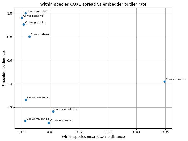
By contrast, some species were comparatively coherent in both molecular and embedding space. Conus maioensis showed low within-species COX1 variation (mean 0.001214; maximum 0.003145), a low outlier rate (0.083333), and high same-class neighborhood purity (0.893632), despite the embedder flagging it as a split candidate. Conus ermineus also remained relatively coherent in embedding space, with a low outlier rate (0.068173) and very high same-class neighborhood purity (0.905575), even though its within-species COX1 variation was appreciably higher than that of C. maioensis (mean 0.009404; maximum 0.014212). These cases indicate that increased mitochondrial variation does not inevitably translate into image-space instability, and that some taxa can remain morphologically coherent despite broader COX1 dispersion.
Table 12. Correlation summary for species-level concordance analyses
| Comparison | Pearson correlation | Spearman correlation |
|---|---|---|
| Mean within-species COX1 distance vs embedder outlier rate | -0.242970 | -0.483333 |
| Minimum COX1 distance to nearest species vs mean same-class kNN fraction | 0.642353 | 0.389925 |
Table 12. Correlation summary for the main species-level concordance analyses. Negative values indicate that higher COX1 dispersion tends to be associated with lower embedding coherence, whereas positive values indicate that stronger mitochondrial separation tends to coincide with higher same-class neighborhood purity.
Two additional taxa were especially informative because they highlighted different forms of partial concordance. Conus venulatus showed comparatively high within-species mitochondrial variation (mean 0.010915; maximum 0.029703), yet only a moderate embedder outlier rate (0.164600) and fairly strong neighborhood purity (0.779707). This suggests that substantial COX1 variation can coexist with a largely coherent image-space signal, although the embedder still identified C. venulatus as a split candidate. In contrast, C. trochulus showed low mean mitochondrial dispersion (0.001423) but a broader maximum within-species distance (0.012376), together with a moderate outlier rate (0.262791) and intermediate neighborhood purity (0.580744). Thus, C. trochulus appears more heterogeneous in embedding space than would be expected from its low mean COX1 spread alone, although its broader internal maximum distance and split-candidate status suggest that some structured heterogeneity may nevertheless be present.
The strongest mitochondrial outlier in the current species-level comparison was Conus infinitus. The two available COX1 sequences were highly divergent from one another (mean and maximum within-species distance both 0.049759), and the species also showed only moderate embedding coherence, with an outlier rate of 0.420168 and a same-class neighborhood purity of 0.444706. Although this taxon is represented by only two sequences and therefore remains descriptive rather than stable at the molecular level, it stands out as the clearest case in which elevated mitochondrial spread and reduced embedding coherence occur in the same direction.
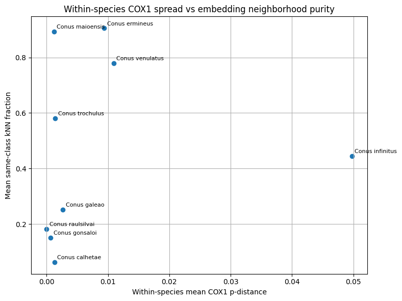
Across species, the relationship between mean within-species COX1 distance and embedder outlier rate was not strongly positive (Table 12). Instead, the correlation was weakly negative by Pearson’s coefficient (r = -0.242970) and moderately negative by Spearman’s rank coefficient (ρ = -0.483333), indicating that species with greater mitochondrial dispersion did not systematically show higher image-space outlier rates. This result is consistent with the visual pattern in which several low-dispersion taxa occupy the highest outlier-rate region, while some taxa with broader COX1 spread remain comparatively coherent in embedding space. By contrast, the relationship between mitochondrial separation from the nearest other species and same-class neighborhood purity was more positive (Pearson r = 0.642353; Spearman ρ = 0.389925), indicating that taxa more strongly separated from their nearest mitochondrial neighbors tended, on average, to show cleaner embedding neighborhoods (Figure 4, Table 12).
Taken together, these species-level results indicate that concordance between COX1 variation and embedding diagnostics is real but incomplete. Concordant taxa, such as Conus maioensis and to a lesser extent C. infinitus, support the interpretation that embedding structure can reflect biologically meaningful signal. However, the strongly discordant behavior of taxa such as C. calhetae, C. gonsaloi, C. raulsilvai, and C. galeao shows that image-space instability cannot be explained by mitochondrial variation alone. In this sense, the molecular evidence functions as an orthogonal plausibility signal: agreement between DNA and embedding strengthens confidence that the embedding space captures biologically relevant structure, whereas disagreement highlights cases that warrant closer inspection for imaging artifacts, label noise, or unresolved biological complexity rather than automatic taxonomic revision.
Concordance between mitochondrial distances and embedding diagnostics - Pairwise concordance between interspecific COX1 distance and embedding cross-class proximity
At the species-pair level, concordance between mitochondrial distance and embedding-based cross-class proximity was present in some cases but was not consistent across the full set of comparisons (Table 13). Some of the strongest cross-class proximities in embedding space involved species pairs that were also close in COX1 space, supporting the interpretation that at least part of the embedding confusion reflects biologically plausible relatedness. However, several other pairs were very close in embedding space despite substantial mitochondrial separation, indicating that image-space proximity cannot be explained by COX1 similarity alone.
Table 13. Top embedding cross-class pairs with corresponding COX1 distances
| Species pair | Embedder cross-class pairs | Minimum embedder cross-class distance | Mean embedder cross-class distance | Minimum interspecific COX1 distance | Mean interspecific COX1 distance |
|---|---|---|---|---|---|
| Conus raulsilvai – Conus trochulus | 84 | 0.015921 | 0.032787 | 0.099010 | 0.102157 |
| Conus trochulus – Conus venulatus | 95 | 0.017430 | 0.032022 | 0.000000 | 0.014891 |
| Conus ermineus – Conus venulatus | 129 | 0.019456 | 0.034191 | 0.103960 | 0.114785 |
| Conus raulsilvai – Conus venulatus | 28 | 0.020440 | 0.032563 | 0.099010 | 0.107363 |
| Conus ermineus – Conus trochulus | 23 | 0.021317 | 0.032835 | 0.104863 | 0.114660 |
| Conus ermineus – Conus raulsilvai | 12 | 0.022706 | 0.031045 | 0.127261 | 0.131811 |
| Conus calhetae – Conus galeao | 1 | 0.023653 | 0.023653 | 0.002584 | 0.004072 |
| Conus infinitus – Conus trochulus | 11 | 0.024607 | 0.033830 | 0.096535 | 0.100391 |
| Conus infinitus – Conus maioensis | 5 | 0.026525 | 0.033049 | 0.051887 | 0.058506 |
| Conus gonsaloi – Conus trochulus | 3 | 0.029116 | 0.032086 | 0.096535 | 0.100554 |
Table 13. Ranked cross-class embedding pairs with corresponding interspecific COX1 distances. Smaller embedder distances indicate stronger cross-class proximity in image space. Comparing these values with mitochondrial distances allows assessment of whether embedding confusion is concordant with biological proximity.
The clearest concordant case was the pair Conus trochulus–C. venulatus (Table 14). This pair showed strong cross-class proximity in embedding space (minimum embedder cross-class distance 0.017430; mean 0.032022) and was also the closest pair in the mitochondrial dataset, with a minimum interspecific COX1 distance of 0.000000 and a mean interspecific distance of 0.014891. This combination indicates that the prominent image-space proximity between these taxa is compatible with very close mitochondrial relationships. A second concordant case was C. calhetae–C. galeao, which showed both low embedding separation (minimum 0.023653) and very low mitochondrial distance (minimum 0.002584; mean 0.004072). Likewise, C. gonsaloi–C. raulsilvai formed another concordant close pair, combining low cross-class embedding distance with very low interspecific COX1 divergence (minimum 0.003230; mean 0.003543). Together, these pairs support the interpretation that some of the strongest cross-class proximities recovered by the embedder correspond to biologically plausible nearest-neighbor relationships rather than purely technical or labeling artifacts.
Table 14. Illustrative concordant and discordant pairwise cases
| Category | Species pair | Minimum embedder cross-class distance | Minimum interspecific COX1 distance | Mean interspecific COX1 distance |
|---|---|---|---|---|
| Concordant close | Conus trochulus – Conus venulatus | 0.017430 | 0.000000 | 0.014891 |
| Concordant close | Conus calhetae – Conus galeao | 0.023653 | 0.002584 | 0.004072 |
| Concordant close | Conus gonsaloi – Conus raulsilvai | 0.032005 | 0.003230 | 0.003543 |
| Discordant | Conus raulsilvai – Conus trochulus | 0.015921 | 0.099010 | 0.102157 |
| Discordant | Conus ermineus – Conus venulatus | 0.019456 | 0.103960 | 0.114785 |
| Discordant | Conus ermineus – Conus trochulus | 0.021317 | 0.104863 | 0.114660 |
Table 14. Selected pairwise cases illustrating agreement and disagreement between image-space cross-class proximity and mitochondrial distance. Concordant pairs are close in both embedding and COX1 space, whereas discordant pairs are close in embedding space despite substantial mitochondrial separation.
At the same time, the pairwise comparison also revealed several strongly discordant cases. The smallest embedder cross-class distance in the ranked set was observed for Conus raulsilvai–C. trochulus (0.015921), yet this pair was not close in mitochondrial space, with a minimum interspecific COX1 distance of 0.099010 and a mean distance of 0.102157. Similarly, C. ermineus–C. venulatus and C. ermineus–C. trochulus both showed strong cross-class proximity in embedding space (minimum distances 0.019456 and 0.021317, respectively), despite substantial mitochondrial separation in both cases (minimum interspecific distances 0.103960 and 0.104863, respectively). These discordant pairs indicate that strong image-space proximity can occur even between taxa that are clearly separated by COX1, implying that shell morphology, imaging conditions, residual label noise, or unresolved non-mitochondrial biological complexity may all contribute to embedding confusion.
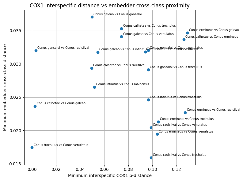
Intermediate cases were also present. For example, Conus infinitus–C. maioensis showed relatively low cross-class embedding distance (minimum 0.026525; mean 0.033049), while their mitochondrial separation was moderate rather than extreme (minimum 0.051887; mean 0.058506). In contrast, C. infinitus–C. trochulus and C. gonsaloi–C. trochulus also showed fairly low embedding distances, but both pairs were much more clearly separated in COX1 space, with minimum interspecific distances near 0.096–0.097. These cases reinforce that pairwise embedding proximity spans a continuum from biologically plausible closeness to clear DNA–embedding disagreement.
Across all species pairs represented in both data layers, the global relationship between minimum interspecific COX1 distance and minimum embedder cross-class distance was weak (Figure 5). Pearson correlation was close to zero (r = 0.016309), and Spearman rank correlation was slightly negative (ρ = -0.098719). Thus, at the pairwise level, species pairs that were especially close in embedding space were not consistently those with the smallest mitochondrial distances. This weak global association contrasts with the existence of several highly informative individual concordant pairs, indicating that the relationship between DNA and embedding structure is driven more by specific taxon pairs than by a simple monotonic trend across the dataset as a whole.
Taken together, these pairwise results show that embedding-based cross-class proximity contains both biologically meaningful and non-concordant components. Concordant close pairs such as Conus trochulus–C. venulatus, C. calhetae–C. galeao, and C. gonsaloi–C. raulsilvai support the view that the embedding space can recover relationships that are also reflected in mitochondrial similarity. By contrast, strongly discordant pairs such as C. raulsilvai–C. trochulus and the C. ermineus pairings demonstrate that image-space confusion may also arise despite substantial COX1 divergence. In this sense, the pairwise mitochondrial analysis does not function as an automatic decision rule, but rather as an external plausibility check that helps distinguish embedding confusions consistent with biological proximity from those more likely to reflect imaging artifacts, label noise, or unresolved morphological complexity.
Discussion
A reproducible benchmark for human-led species triage
The central contribution of this study is not an automated claim to “discover” species directly from images, but the development of a reproducible benchmark for human-led triage in species delimitation workflows. In this framework, the embedding model is used as a decision-support instrument rather than as a taxonomic oracle. Its role is to organize heterogeneous shell imagery into a structured set of diagnostic signals that can guide expert review, including measures of within-species cohesion, outlier burden, nearest-neighbor interference, cross-class proximity, and stability across repeated resampling or bootstrap conditions. A fuller methodological discussion of embedding-based quantitative morphology, including its advantages and interpretive limits for shell-taxonomic review, is provided as a Supplement [Supp. 2]. The purpose of the system is therefore not to replace taxonomic judgement, but to make review more systematic, more transparent, and more scalable. [29]
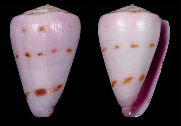
This distinction matters because species delimitation in collector and museum imagery is affected by multiple sources of complexity that cannot be resolved by a single model output alone. Historical label drift, synonymy, variable imaging conditions, uneven representation of morphotypes, and true biological heterogeneity can all produce similar apparent patterns in image space. A workflow that simply converts clustering or embedding proximity into automatic split/lump decisions risks overinterpreting these signals. By contrast, the present benchmark is explicitly designed to separate different kinds of cases: compact taxa that remain stable under repeated evaluation, heterogeneous taxa that deserve closer review, outlier-rich groups that may contain imaging artifacts or mislabeled material, and problematic species pairs whose repeated proximity suggests either biological relatedness or persistent ambiguity. This makes the output operationally useful even when the final taxonomic interpretation remains unresolved [20].
A further strength of the benchmark is that it evaluates not only central tendency but also consistency. Rather than relying on a single embedding arrangement or one-off ranking, the workflow quantifies which species and species pairs are repeatedly recovered as compact, unstable, suspicious, or close across repeated analyses. This shifts the emphasis from anecdotal visual impressions to reproducible triage signals. In practice, such reproducibility is valuable because it allows researchers to prioritize finite expert time toward the cases most consistently identified as problematic, while assigning greater confidence to taxa that remain coherent and well separated across repeated runs.
The benchmark therefore contributes a middle ground between fully manual curation and overconfident automated delimitation. It provides a structured review layer in which embeddings are used to surface interpretable patterns, not to finalize taxonomic acts. In that sense, the main advance of the present study is methodological rather than taxonomic: it establishes a framework for identifying where human attention should be directed, why those cases were flagged, and how stable those flags remain under repeated evaluation. This is particularly relevant for groups such as Cabo Verde Conus, where morphological variation, synonymy, and image-source heterogeneity make binary automated decisions especially risky.
Why stability and uncertainty matter for curation
A key strength of the present workflow is that it evaluates not only which taxa or species pairs are flagged, but also how consistently they are flagged across repeated analyses. This is scientifically important because single-run embedding outputs can be sensitive to sampling composition [47], stochastic variation, and the particular arrangement of images included in a given run [48]. In a one-shot analysis, a species may appear compact, unstable, or suspicious simply because of a transient configuration of specimens rather than because the underlying signal is genuinely robust. By incorporating repeated-run stability and bootstrap-based resampling, the benchmark moves beyond a single ranking or visualization and instead asks whether the same taxa repeatedly emerge as coherent, problematic, or ambiguous under perturbed conditions.
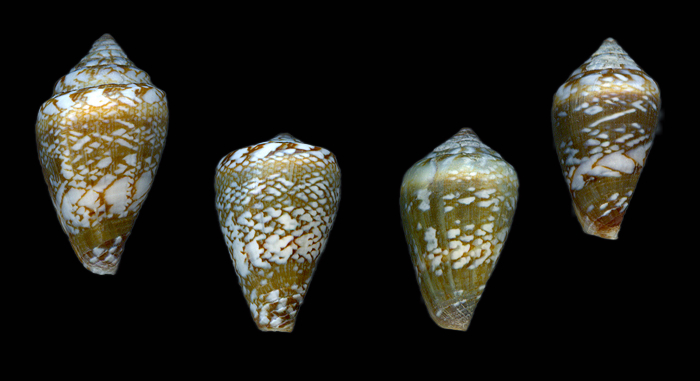
This uncertainty layer makes the workflow more defensible in both scientific and operational terms. Scientifically, persistence across repeated runs provides a stronger basis for interpretation than isolated extreme values. A taxon that repeatedly appears among the most unstable groups, or a species pair that repeatedly appears among the closest cross-class pairs, is much more likely to represent a meaningful pattern than a taxon or pair that is flagged only once. Metrics such as bootstrap persistence, Top-10 persistence, and worst-rank frequency therefore serve as measures of reproducibility rather than simple point estimates. They help distinguish robust signals from unstable ones and reduce the risk of overinterpreting one-off artifacts in the embedding space.
Operationally, these stability measures are equally valuable because they support prioritization. In a realistic curation setting, expert time is limited, and not every suspicious case can be reviewed immediately. A ranked list based only on a single analysis does not adequately distinguish between consistently problematic taxa and cases that are sensitive to minor perturbations. By contrast, a species that is repeatedly flagged across bootstrap replicates and repeatedly reappears among the most heterogeneous or interference-prone taxa represents a stronger candidate for urgent review. Stability-aware ranking thus improves triage efficiency: it helps direct attention first toward the taxa and species pairs whose problematic behavior is not merely extreme, but persistent.
The value of uncertainty quantification is especially clear in a system such as the Cabo Verde Conus assemblage, where multiple biological and technical factors can interact. Variable shell morphology, uneven image quality, mixed sources, historical synonymy, and label inconsistency may all influence the embedding structure. Under such conditions, it is risky to interpret the output of a single run as if it were definitive. Repeated evaluation does not remove that complexity, but it makes its effects more visible. Cases that remain unstable across repeated perturbations become more credible curation targets, while cases that fluctuate widely may indicate marginal signals or sensitivity to sparse sampling. In this way, uncertainty is not treated as a nuisance to be hidden, but as part of the information needed for responsible interpretation.
More broadly, the use of repeated-run and bootstrap-based metrics helps align the workflow with the actual needs of human-led curation. The goal is not merely to assign a score, but to provide evidence that a score is sufficiently stable to justify expert attention. This shift from raw ranking to reproducible ranking is one of the benchmark’s main methodological advances. It makes the workflow more transparent, more auditable, and less dependent on a single arbitrary run, thereby strengthening its value as a defensible decision-support system rather than a fragile exploratory analysis.
Species-level interpretation: compact taxa versus unstable taxa
One of the most informative outcomes of the present benchmark is that poor embedding behavior is not reducible to a single biological or technical cause. At the species level, some taxa were compact and coherent in both mitochondrial and image space, whereas others were highly unstable in embedding space despite showing little COX1 dispersion. This mixed pattern supports the broader integrative-taxonomy view that no single data source should be treated as definitive in isolation and that species-level interpretation is strongest when morphology, molecular evidence, and other signals are evaluated jointly [29].
The compact taxa are important because they show what a biologically and curatorially reassuring signal looks like in this framework. Species such as Conus maioensis combined low within-species COX1 spread with relatively coherent embedding behavior, while C. ermineus remained embedding-coherent despite broader mitochondrial variation. In practical terms, these taxa are the easiest to curate: they are less likely to require immediate large-scale review, and they provide reference examples of how a stable species behaves when both molecular and embedding evidence broadly agree. Such cases strengthen the argument that the benchmark can recover meaningful biological structure rather than merely ranking noise [30].
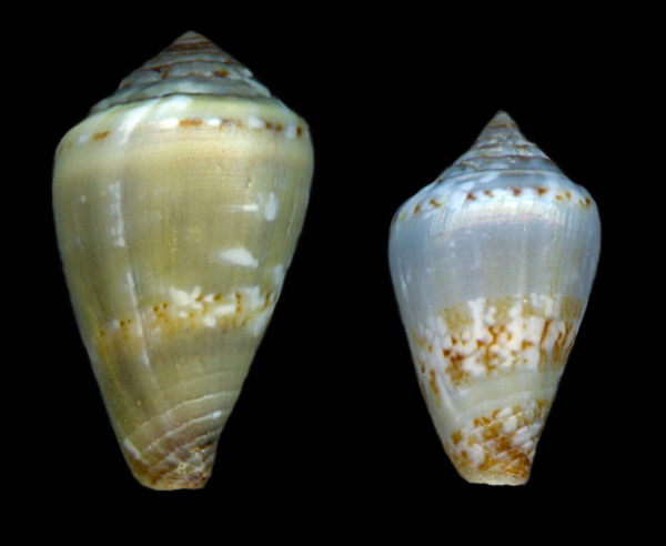
By contrast, taxa such as C. calhetae, C. gonsaloi, C. raulsilvai, and C. galeao are especially important because they show that strong embedding instability can coexist with very low COX1 dispersion. These are not simple “high-variation species” in a mitochondrial sense, yet they behave as heterogeneous or outlier-rich groups in image space. Scientifically, that makes them high-value review targets rather than failures of the workflow. Curatorially, they are exactly the taxa for which a human-led triage system is most useful, because they likely concentrate a mixture of causes: residual label noise, image-source heterogeneity, inconsistent specimen presentation, subtle but nonrandom morphotype structure, or biologically meaningful variation not well tracked by mitochondrial COX1 alone. Integrative-taxonomy studies repeatedly show that discordance among evidence types is common and that mitochondrial markers may fail to mirror morphological or nuclear structure in a simple one-to-one manner [30].
This is also why the unstable taxa should not be interpreted automatically as evidence for hidden species, nor dismissed automatically as noise. A taxon with high embedding outlier burden but low COX1 spread may reflect technical artifacts, but it may also reflect unresolved morphological complexity that is real at the phenotypic level yet weakly captured by a single mitochondrial marker. Conversely, a taxon with elevated COX1 spread and reduced embedding coherence, such as C. infinitus in the current dataset, may represent a more biologically plausible candidate for deeper review, although the current molecular sample size remains too small for strong inference. The key point is that instability becomes actionable because it directs attention, not because it delivers a taxonomic verdict. That interpretation is closely aligned with integrative delimitation frameworks that treat discordant evidence as a cue for targeted follow-up rather than an obstacle to be ignored [31].
From a curation perspective, the distinction between compact and unstable taxa is one of the most operationally useful outputs of the benchmark. Compact taxa can function as relatively secure anchors in the dataset, while unstable taxa define the highest-priority review queue. In that sense, the benchmark adds value even when it does not resolve the biological cause of instability immediately. It helps partition the dataset into species that are currently well behaved, species that are persistently problematic, and species that warrant escalation to more targeted molecular, morphological, or metadata-based review [30]. This is exactly where a decision-support framework is most useful: not in replacing expert judgement, but in making the location and likely nature of ambiguity more visible and more reproducible.
Pairwise interpretation: biologically plausible confusion versus discordant confusion
The pairwise results show that cross-class proximity in embedding space is biologically interpretable, but not uniformly so. Some of the closest species pairs in image space were also among the closest pairs in COX1 space, which supports the view that the embedding model can recover relationships that are at least partly consistent with biological relatedness. At the same time, other pairs were very close in embedding space despite substantial mitochondrial separation, indicating that image-space confusion is not equivalent to genetic proximity and should not be treated as a split/lump rule on its own. This mixed outcome is consistent with the broader integrative-taxonomy literature, which emphasizes that agreement among data layers can be highly informative, whereas disagreement is common and often biologically or curatorially meaningful rather than simply “wrong.”
The concordant close pairs are especially important because they demonstrate that the benchmark is capable of identifying confusion candidates that are biologically plausible rather than merely visually similar. In the present dataset, pairs such as Conus trochulus–C. venulatus, C. calhetae–C. galeao, and C. gonsaloi–C. raulsilvai were close in both embedding and mitochondrial space. These cases strengthen confidence that some cross-class proximities in the embedding results are not arbitrary artifacts of image presentation, but instead reflect relationships that are also visible in the molecular data. In a curation context, such concordant pairs are useful because they identify the species pairs for which embedding confusion is most likely to correspond to genuine biological proximity and therefore deserves more nuanced review rather than immediate correction.
Equally important, however, are the discordant pairs. Several species pairs were among the strongest cross-class neighbors in embedding space despite being well separated in COX1 space. These cases indicate that strong image-space proximity may arise from sources other than simple mitochondrial relatedness, including convergent or overlapping shell morphology, image-source heterogeneity, historical label inconsistency, or biological complexity not captured by a single mitochondrial marker. In this sense, discordant confusion is not a failure of the benchmark; rather, it is one of its most useful outputs. It highlights precisely those species pairs for which morphology-like signal in image space and mitochondrial signal diverge, thereby identifying cases where expert review is most needed. That interpretation is aligned with work on mitonuclear discordance and integrative delimitation [31], where conflicting signal among morphology, mtDNA, and other evidence types is treated as a prompt for hypothesis testing rather than a reason to privilege one source automatically.
From a practical perspective, the pairwise benchmark therefore helps partition confusion into at least two classes. The first consists of biologically plausible confusion pairs, where image-space and mitochondrial proximity point in the same direction. The second consists of discordant confusion pairs, where the embedder repeatedly places species close together despite strong mitochondrial separation. This partition is curatorially valuable because the two classes imply different follow-up actions. Concordant close pairs may warrant careful review of boundaries, broader sampling, or additional loci, whereas discordant pairs may more strongly motivate inspection of image quality, metadata, label provenance, and morphology-specific sources of ambiguity. The workflow thus turns a generic notion of “confusion” into a more interpretable and actionable signal.
More broadly, the pairwise results reinforce the paper’s central claim that embeddings are best understood as a decision-support layer rather than as an autonomous delimitation engine. When cross-class proximity is concordant with mitochondrial proximity, it increases confidence that the embedding space is recovering biologically meaningful structure. When the two signals disagree, the disagreement itself becomes informative: it marks a pair for further scrutiny, suggests that a single-locus mitochondrial interpretation may be incomplete, or indicates that image-space ambiguity has a non-molecular source. In this way, pairwise interpretation is not about deciding which signal is “correct,” but about using concordance and discordance to prioritize review and refine hypotheses. That is exactly the role an integrative, human-led delimitation workflow should play
The role and limits of COX1 as an orthogonal validation layer
The mitochondrial component of this study is most useful as an external plausibility check rather than as an autonomous species-delimitation criterion. COX1 has long been valuable for animal identification and often provides strong discriminatory power among closely related taxa, which makes it a reasonable orthogonal signal for evaluating whether embedding-based proximity is biologically plausible [24].
In that sense, the main value of COX1 here is not that it can decide species boundaries by itself, but that it can help interpret the meaning of patterns recovered in image space. When species are close in both embedding and mitochondrial space, confidence increases that the embedding signal reflects genuine biological relatedness rather than only visual similarity or technical artifact [30].
At the same time, the present dataset also makes clear what mitochondrial DNA cannot do in this framework. COX1 coverage is uneven across the accepted species, with some taxa represented by many sequences and others by only one or two, so the molecular layer is not equally informative across the full Maio assemblage. Under such conditions, mtDNA is best interpreted as a partial validation subset rather than as comprehensive molecular coverage of the focal fauna.
This limitation is especially important for interpreting the discordant cases recovered in the present study. A species or species pair that is unstable or unusually close in embedding space, yet not close in COX1 space, should not automatically be dismissed as a false positive, just as a close mitochondrial relationship should not automatically be interpreted as proof of taxonomic lumping. Rather, such cases should be treated as candidates for deeper review using additional evidence, including morphology, metadata, broader sampling, or nuclear markers where possible [31].
The discussion therefore returns to the same principle established in the Introduction and Methods: mitochondrial DNA is informative because it provides an independent line of evidence, but its role in this study is supportive rather than decisive. It helps distinguish embedding patterns that are more biologically plausible from those that are more suspicious or more difficult to interpret, yet it does not replace the need for human judgement or integrative follow-up.
Overall, the strength of the mitochondrial layer lies precisely in this limited but important role. COX1 improves interpretability, sharpens prioritization, and provides external biological context for the benchmark, but it cannot adjudicate every difficult case on its own, nor should it be expected to do so in an integrative delimitation workflow.
Why DNA–embedding discordance is informative
A central implication of the present study is that discordance between mitochondrial and embedding-based structure should not be interpreted primarily as a weakness of the workflow. In integrative delimitation, disagreement among data layers is common and is often one of the most informative outcomes, because it identifies the taxa or species pairs for which a simple, single-source explanation is inadequate [38].
Within that perspective, discordant taxa become especially valuable because they concentrate biological and curatorial uncertainty in a tractable set of review targets. A species that is compact in COX1 space but unstable in embedding space, or a species pair that is close in image space despite substantial mitochondrial separation, is not merely an “error case.” Instead, it is a case in which different evidence layers are capturing different aspects of the underlying system, thereby indicating where expert attention is most needed.
This is precisely why the human-led benchmark logic is stronger than a workflow that seeks full automatic agreement. If the goal were simply to maximize concordance, discordant cases would appear as failures to be minimized. In a triage-oriented framework, however, discordance is productive because it helps separate straightforward taxa from those that warrant deeper scrutiny. A discordant taxon may reflect image-source heterogeneity, residual label noise, historical taxonomic instability, morphologically overlapping shells, incomplete lineage sorting, introgression, or other forms of biological complexity not captured by a single mitochondrial marker.
The results of this study illustrate that point clearly. Several taxa were unstable in embedding space despite low within-species COX1 dispersion, while some strongly proximate cross-class embedding pairs remained well separated in mitochondrial space. These patterns are scientifically useful because they identify exactly where a one-dimensional interpretation would be misleading. Rather than forcing a premature split/lump decision, the workflow makes these cases visible and reproducible, allowing them to be escalated for targeted follow-up. Such follow-up may include closer morphological review, metadata checking, image-quality inspection, additional specimen sampling, or the incorporation of nuclear markers and broader integrative evidence.
In this sense, discordance is not an obstacle to interpretation but part of the interpretation itself. Concordant cases show where the workflow is capturing biologically plausible structure across evidence layers, whereas discordant cases mark where that structure is incomplete, mixed, or potentially confounded. The benchmark is therefore useful not because it eliminates ambiguity, but because it localizes ambiguity in a systematic and defensible way.
Framed this way, discordance becomes one of the paper’s strongest outcomes. It supports the broader claim that species delimitation in heterogeneous image datasets should be approached as an evidence-integration problem rather than as a search for a single decisive signal. The practical value of the workflow lies in its ability to convert disagreement into prioritization: taxa and species pairs that remain discordant across embedding and mitochondrial analyses become the highest-value candidates for expert review, not because the system has failed, but because it has successfully identified where biological or curatorial complexity is concentrated.
AI-assisted software development as an accelerator of workflow iteration, with human verification safeguards
An important practical aspect of this study was the use of AI-assisted code generation and iterative prototyping (“vibe coding”) during development of the curation framework and supporting analysis pipeline. In practice, this substantially increased the speed at which workflow ideas could be converted into executable tools, inspected, and revised [1, 2]. For this project, the main benefit was not replacement of domain expertise, but reduction of implementation latency between methodological concepts (e.g., new diagnostics, review queues, or dataset-state transitions) and empirical evaluation within the pipeline.
This acceleration had methodological consequences. Faster implementation and revision cycles made it feasible to explore a broader range of curation-support mechanisms than would typically be practical under a slower manual development process. In particular, the workflow benefited from rapid iteration on user-facing review pages, embedding-diagnostic outputs, and data-pipeline logic connecting metadata, filesystem images, and curated states. This likely improved the operational quality of the framework by allowing earlier detection of design ambiguities and by enabling repeated refinement of how diagnostic evidence is presented for human review [3, 4].
At the same time, AI-assisted coding introduces risks that are directly relevant to scientific software development, including plausible but incorrect implementations, hidden logic errors, and overconfidence in generated code. In this study, these risks were mitigated through human review, test runs on known subsets, and inspection of intermediate outputs, but they remain an important limitation of LLM-assisted development more broadly [Supp. 1]. The usefulness of this approach therefore depends on maintaining a strict distinction between implementation assistance and scientific validation: AI can accelerate coding, but correctness of the analysis pipeline and interpretation of results must remain author-controlled.
More broadly, the experience in this project suggests that AI-assisted development may be especially valuable for iterative, tool-rich biodiversity curation workflows, where progress depends on repeated adjustments to diagnostics, interfaces, and data-state logic rather than on a single fixed software implementation. Under these conditions, the primary impact of LLM assistance may be less about reducing total coding effort and more about increasing the number of high-quality design iterations that can be completed within a given time window. This may, in turn, improve the responsiveness of human-led curation workflows, provided that validation and auditability remain central.
Limitations of the current study
Several limitations of the present dataset and benchmark should be made explicit. First, the mitochondrial component is unevenly sampled across accepted taxa, and that unevenness is not a minor technical detail but a genuine interpretive constraint. Public barcode resources are often taxonomically and geographically incomplete, with strong variation in sequence density among lineages and substantial gaps in coverage, which limits the extent to which mtDNA can be treated as a balanced comparative layer across all taxa [33].
That broader limitation is visible in the current study, where some species are represented by many COX1 sequences whereas others are represented by only one or two. As a result, within-species mitochondrial summaries are substantially more informative for some taxa than for others, and several species contribute mainly to interspecific comparison rather than to robust estimates of internal mitochondrial dispersion. This means that the DNA component is best viewed as a partial validation subset rather than as a complete molecular characterization of the Maio assemblage.
A second limitation concerns the image data themselves. Collector and museum-style image datasets are inherently heterogeneous, and machine-learning performance in such settings depends strongly on data curation, metadata quality, and the degree to which images differ in presentation, provenance, and associated recording practices. Studies on machine learning with museum collections emphasize that standard assumptions often do not transfer cleanly to collection-derived datasets, and that erroneous entries, missing values, inconsistent metadata, and variable imaging conditions can all propagate downstream into model behavior [34].
This image heterogeneity is particularly relevant in the present benchmark because the workflow is intentionally designed to surface outlier-rich taxa and unstable neighborhoods. Some of those signals are likely to reflect biologically meaningful structure, but others may arise from mixed image sources, inconsistent specimen presentation, or other curatorial artifacts. The benchmark is useful precisely because it identifies such cases, but the existence of those cases also means that not all embedding instability should be interpreted biologically in the first instance.
A third limitation involves taxonomic consistency in historical names and source records. Biodiversity datasets assembled from multiple repositories and historical sources routinely contain heterogeneity in taxon names, heterogeneity in taxonomic concepts, and uncertainty in the accuracy of identifications, all of which can affect downstream analyses if they are not actively harmonized [35].
Although the present study explicitly groups sequences by accepted names and applies name normalization, such harmonization cannot eliminate all residual uncertainty. Synonymized names, historically shifting species concepts, and differences in source-level identifications may still leave traces in the dataset, particularly in controversial groups or lineages with recent diversification. More generally, name-resolution studies have shown that inconsistent or outdated taxon naming can substantially distort biodiversity analyses if used uncritically [36].
A fourth limitation is the scope of the benchmark itself. The Maio Conus system is a strong testbed because it combines geographic constraint, dense local taxonomic complexity, heterogeneous imagery, and biologically meaningful ambiguity, but it remains a constrained case study rather than a comprehensive representation of the genus or of molluscan image-based delimitation more broadly. The present benchmark therefore demonstrates that the workflow is useful in one challenging regional radiation, but it does not by itself establish that the same performance characteristics, stability patterns, or DNA–embedding relationships will hold unchanged across other islands, broader Cabo Verde assemblages, or other gastropod groups.
For that reason, the benchmark should be interpreted as a deliberately focused proof of utility rather than as a universal solution. Its strength lies in showing that a human-led, stability-aware triage workflow can generate biologically interpretable and curatorially useful signals under realistic conditions of heterogeneity and partial molecular coverage. Its limitation is that those signals remain conditioned by uneven DNA availability, source heterogeneity, residual naming uncertainty, and the bounded taxonomic scope of the current test system. Those constraints do not undermine the value of the study, but they do define the context in which its conclusions should be interpreted.
Implications for future integrative delimitation workflows
Several next steps follow directly from the present benchmark. The first is targeted molecular follow-up for the taxa and species pairs that were most consistently flagged as unstable, suspicious, or discordant across the embedding and COX1 analyses. Rather than seeking blanket molecular expansion across the full dataset immediately, a more efficient strategy is to prioritize those species and pairwise relationships that repeatedly reappear in bootstrap persistence, Top-10 persistence, worst-rank frequency, or pairwise cross-class proximity summaries, because these are the cases where additional evidence is most likely to change interpretation. This kind of targeted validation is well aligned with current integrative-delimitation thinking, which emphasizes iterative hypothesis testing rather than one-pass species assignment.
A second priority is to extend the molecular layer beyond mitochondrial COX1 in the most problematic cases. Where image-space structure and COX1 agree, the present workflow already provides a useful plausibility signal, but discordant taxa and species pairs would benefit from nuclear markers or broader genomic sampling. Recent reviews emphasize that genomic and multilocus data are particularly valuable when mtDNA-based interpretation is ambiguous or when mito-nuclear discordance is suspected, because they separate the discovery of candidate units from the validation of species boundaries more effectively than a single mitochondrial marker alone [37].
A third direction is expansion of the benchmark itself. The Maio Conus assemblage is a strong regional testbed, but the real value of the framework will be clearer once the same workflow is applied across additional islands and broader Cabo Verde assemblages. Expanding geographically would test whether the same stability patterns, confusion structures, and discordance profiles recur under wider sampling, and would also make it possible to distinguish local from archipelago-wide ambiguity. More generally, recent discussions of “species delimitation 4.0” argue that the combination of integrative taxonomy and AI-based feature learning becomes most powerful when workflows can be scaled and compared across broader datasets rather than remaining isolated to a single local system [27].
A fourth and more operational direction concerns refinement of seed lists and review queues. One of the most useful outputs of the current benchmark is that it does not merely flag problematic taxa once; it identifies which taxa and species pairs are repeatedly problematic across bootstrap and pairwise analyses. That information can be used directly to improve the workflow itself by revising seed definitions, inspecting recurrent outlier-rich sources, separating morphotype-like clusters for review, or restructuring the human-review queue around persistence rather than one-off rank position. In this sense, the benchmark can become self-improving: repeated instability does not merely identify a biological question, but also guides how the next round of curation and model evaluation should be designed
A final future direction is methodological integration rather than simple data expansion. The strongest long-term value of the present framework will likely come from using embeddings, mitochondrial summaries, nuclear follow-up, metadata review, and expert morphology together as linked evidence streams rather than as separate analyses. Integrative taxonomy has long argued that difficult delimitation problems are best approached by combining complementary data types in a transparent, iterative framework, and the present benchmark provides a practical structure for doing exactly that in heterogeneous shell-image datasets [23].
Overall, the most promising path forward is therefore not simply to collect more data, but to collect the right additional data for the right flagged cases [32], while expanding the benchmark in a way that preserves its central strengths: human-led review, explicit uncertainty, reproducible ranking, and interpretable integration across evidence layers [20, 23].
References
- [1] J.G. Meyer. Rapid Development of Omics Data Analysis Applications through Vibe Coding. arXiv:2510.09804 [q-bio.OT] (2025)
- [2] Baek E, Ju HJ, Seo J, Yoon JY.. A Vibe Coding Workflow for AI-Assisted Analysis and Visualization of Genbank Records of Pepper Infecting Viruses.. Plant Pathol J. 42(1):103–108 (2026)
- [3] Cui, Z. K. et al. The effects of generative AI on high-skilled work: Evidence from three field experiments with software developers. Management Science 0(0) (2026)
- [4] N. Cheimarios. Scientific software development in the AI era: reproducibility, MLOps, and applications in soft matter physics. Front. Phys., Sec. Soft Matter Physics Volume 13 (2025)
- [5] Cock, PJ et al. Biopython: freely available Python tools for computational molecular biology and bioinformatics. Bioinformatics, 25(11), 1422–1423. (2009)
- [6] Zhang, Q., Zhou, J., He, J. et al. A shell dataset, for shell features extraction and recognition. Nature, Sci Data 6, 226 (2019)
- [7] MJ Tenorio et al. Taxonomic revision of West African cone snails (Gastropoda: Conidae) based upon mitogenomic studies: implications for conservation. European Journal of Taxonomy, (663). (2020)
- [8] M Tan and Quoc V. Le. EfficientNetV2: Smaller Models and Faster Training. Proceedings of the 38th International Conference on Machine Learning, (2021)
- [9] Bardes A, Ponce J, LeCun Y. VICReg: Variance-Invariance-Covariance Regularization for Self-Supervised Learning. International Conference on Learning Representations (ICLR) (2022)
- [10] Russakovsky O et al. ImageNet Large Scale Visual Recognition Challenge. International Journal of Computer Vision 115:211–252 (2015)
- [11] Ester M, et al. A Density-Based Algorithm for Discovering Clusters in Large Spatial Databases with Noise.. Proceedings of the Second International Conference on Knowledge Discovery and Data Mining p. 226–231. (1996)
- [12] Rolán E. Descripción de nuevas especies y subespecies del género Conus (Mollusca, Neogastropoda) para el Archipiélago de Cabo Verde. . Iberus, Supplement 2: 5–70 (1990)
- [13] P. Kersten Cone Collector's Guide. The Cone Collector (2015)
- [14] Afonso C.M.L. & Tenorio M.J. Recent findings from the islands of Maio and Boa Vista in the Cape Verde Archipelago, West Africa: description of three new Africonus species (Gastropoda: Conidae).. Xenophora Taxonomy 3: 47–60 (2014)
- [15] Tenorio M.J. & Afonso C.M.L. Description of four new species of Conus from the Cape Verde Islands (Gastropoda, Conidae.). Visaya 2: 24–37 (2004)
- [16] Cossignani T. & Fiadeiro R. Africonus perrineae: un nuovo cono da Capo Verde. Malacologia Mostra Mondiale 99: 17–19 (2018)
- [17] G Van Horn et al. The iNaturalist Species Classification and Detection Dataset arXiv:1707.06642 [cs.CV] (2017)
- [18] C. G. Northcutt, L. Jiang, I. L. Chuang. Confident Learning: Estimating Uncertainty in Dataset Labels. arXiv:1911.00068 [stat.ML] (2019)
- [19] A Radford et al. Learning Transferable Visual Models From Natural Language Supervision. Proceedings of the 38 th International Conference on Machine Learning, PMLR 139, (2021)
- [20] J. D. Hollister et al. A Computer Vision Method for Finding Mislabelled Specimens Within Natural History Collections. Ecology and Evolution, 15:e71648. (2025)
- [21] Peters, H. et al. The cone snails of Cape Verde: marine endemism at a terrestrial scale. Global Change Biology. pp. 201-213 (2016)
- [22] Abalde S., et al. Phylogenetic relationships of cone snails endemic to Cabo Verde based on mitochondrial genomes. BMC Evolutionary Biology 17: 231 (2017)
- [23] B. Dayrat. Towards integrative taxonomy. Biological Journal of the Linnean Society 83(3), 407-415 (2005)
- [24] Hebert PD et al. Biological identifications through DNA barcodes. Proc Biol Sci. 270(1512):313-21 (2003)
- [25] Tayfun Karaderi et al. Visual Microfossil Identification via Deep Metric Learning. arXiv:2112.09490 [cs.CV] (2021)
- [26] P. J. Rousseeuw. Silhouettes: A graphical aid to the interpretation and validation of cluster analysis. Journal of Computational and Applied Mathematics Volume 20, Pages 53-65 (1987)
- [27] Karbstein, K. et al. Species delimitation 4.0: integrative taxonomy meets artificial intelligence. Trends in ecology and evolution. 39, 8, p. 771 - 784. (2024)
- [28] Toews DP, Brelsford A. The biogeography of mitochondrial and nuclear discordance in animals.. Mol Ecol. 21(16):3907-30 (2012)
- [29] Yeates, D.K. et al. Integrative taxonomy, or iterative taxonomy? Systematic Entomology, 36: 209-217 (2011)
- [30] S Papakostas et al. Integrative Taxonomy Recognizes Evolutionary Units Despite Widespread Mitonuclear Discordance: Evidence from a Rotifer Cryptic Species Complex. Systematic Biology, Volume 65, Issue 3, Pages 508–524 (2016)
- [31] Firneno TJ Jr et al. Delimitation despite discordance: Evaluating the species limits of a confounding species complex in the face of mitonuclear discordance. Ecol Evol. 11(18):12739-12753 (2021)
- [32] Tuia, D., Kellenberger, B., Beery, S. et al. Perspectives in machine learning for wildlife conservation. Nat Commun 13, 792 (2022)
- [33] Lo E, Nie R-E and Vogler AP. The geographic and phylogenetic structure of public DNA barcode databases: an assessment using Chrysomelidae (leaf beetles). Front. Ecol. Evol. 12:1305898 (2024)
- [34] L Hughes-Noehrer, J Carlton & C Jay. Machine Learning and Museum Collections: A Data Conundrum. In book: Emerging Technologies and the Digital Transformation of Museums and Heritage Sites (2021)
- [35] Coca-de-la-Iglesia, M. et al. High rate of species misidentification reduces the taxonomic certainty of European biodiversity databases of ivies (Hedera L.).. Sci Rep 14, 4876 (2024).
- [36] Boyle B et al. The taxonomic name resolution service: an online tool for automated standardization of plant names.. BMC Bioinformatics. 14:16. (2013)
- [37] S Singhal et al. A Genomic Perspective on Species Delimitation. Annual Review Ecology, Evolution, and Systematics. 56:467-489 (2025)
- [38] J J. Wiens, T A. Penkrot. Delimiting Species Using DNA and Morphological Variation and Discordant Species Limits in Spiny Lizards (Sceloporus). Systematic Biology, Volume 51, Issue 1, Pages 69–91 (2002)
- [39] L Sluijterman, E Cator, T Heskes How to evaluate uncertainty estimates in machine learning for regression?. Neural Networks Volume 173, 106203 (2024)
- [40] López Carranza N, Carlson SJ. Testing Species Assignments in Extant Terebratulide Brachiopods: A Three-dimensional Geometric Morphometric Analysis of Long-Looped Brachidia. PLoS One. 14(11):e0225528 (2019)
- [41] Liew TS, Schilthuizen M. A Method for Quantifying, Visualising, and Analysing Gastropod Shell Form. PLoS One. 11(6):e0157069 (2016)
- [42] He Y et al. Opportunities and Challenges in Applying AI to Evolutionary Morphology. Integr Org Biol. 6(1):obae036 (2024)
- [43] Ghanegolmohammadi F, Eslami M, Ohya Y. Systematic data analysis pipeline for quantitative morphological cell phenotyping. Comput Struct Biotechnol J. 23:2949-2962 (2024)
- [44] Holvast EJ et al. Do morphometric data improve phylogenetic reconstruction? A systematic review and assessment. BMC Ecol Evol. 24(1):127. (2024)
- [45] RA Lopez Cruz, MJ Pante, FJ Rohlf Geometric Morphometric Analysis of Shell Shape Variation in Conus (Gastropoda: Conidae). Zoological Journal of the Linnean Society 165(2):296-310 (2012)
- [46] F Pedregosa et al. Scikit-learn: Machine Learning in Python. Journal of Machine Learning Research 12 2825-2830 (2011)
- [47] Musgrave, K, Belongie, S and Lim, S. A Metric Learning Reality Check. 16th European Conference on Computer Vision (ECCV), pp 681–699 (2020)
- [48] D Picard. Torch.manual_seed(3407) is all you need: On the influence of random seeds in deep learning architectures for computer vision. arXiv:2109.08203 [cs.CV] (2021)
- [49] F J Rohlf, L F Marcus. A revolution morphometrics. Trends in Ecology & Evolution, Volume 8, Issue 4, Pages 129-132 (1993)
- [50] S Swayamdipta et al. Dataset Cartography: Mapping and Diagnosing Datasets with Training Dynamics. arXiv:2009.10795 [cs.CL]
- [51] Breunig, M M et al. LOF: identifying density-based local outliers. Proceedings of the 2000 ACM SIGMOD International Conference on Management of Data, 93–104 (2000)
Supplementary material
[supp. 1]Supplemental Note 1: Reducing risk in LLM-assisted coding via redundant elicitation and decomposition
Because LLM-assisted coding can produce plausible but incorrect implementations, hidden logic errors, and unwarranted confidence in generated code, I adopted a practical risk-reduction strategy during development of the curation framework and analysis pipeline. This strategy combined (i) divide-and-conquer task decomposition, (ii) re-elicitation of the same coding task using different wording at a later time with the same LLM, and (iii) cross-LLM comparison by asking equivalent questions to a different model.
In the divide-and-conquer step, larger pipeline tasks were decomposed into smaller components (e.g., data retrieval, transformation logic, metric calculation, edge-case handling, and output formatting). This reduced the risk of end-to-end hidden assumptions and made it easier to inspect and test each component independently. For selected components, functionally equivalent code was then re-requested using alternative wording (often separated in time) to obtain a quasi-independent implementation. In some cases, the same task was also posed to a different LLM to obtain an alternative code path. Differences between implementations were treated as diagnostic signals indicating ambiguity, underspecified requirements, or potential logic errors.
This process was used as a risk-reduction and quality-improvement method, not as a replacement for validation. Agreement between independently elicited solutions was considered supportive but not sufficient evidence of correctness, since different LLMs can share common failure modes or converge on similar but incorrect patterns. Therefore, critical components were additionally validated through manual inspection, controlled test cases, and comparison of intermediate outputs (e.g., filtered row counts, selected identifiers, and metric behavior on known subsets).
The main advantages of this approach were improved detection of hidden assumptions, reduced overconfidence in single generated solutions, and faster refinement of specifications and edge-case handling. The main limitations were increased development overhead, potential reproducibility complexity if prompts were repeated across model/version changes, and the fact that code-level agreement does not guarantee correctness of the underlying analytical concept. Accordingly, final methodological definitions and scientific interpretations remained author-controlled and were validated independently of LLM-generated code suggestion
[supp. 2]Supplemental Note 2: Quantitative shell morphology as a reproducible taxonomic signal
Traditional shell taxonomy often depends on expert recognition of shape, sculpture, color pattern, and overall gestalt, but these judgments can be difficult to standardize across large and heterogeneous datasets, especially when specimens originate from mixed historical, collector, and digitized-image sources. Quantitative morphometric approaches were developed in part to address exactly this problem by converting morphological variation into explicit, comparable measurements rather than relying only on qualitative description [49, 40].
This issue is especially relevant for molluscan shells, where form is continuous, highly integrated, and often difficult to summarize fully using a small set of hand-selected characters. Recent work on shell morphometrics has shown that quantitative approaches can provide robust and reproducible descriptions of shell form and can be applied directly to problems in taxonomy, morphology, and evolutionary analysis [41].
Embedding-based analysis offers a quantitative complement by representing shell morphology in a continuous feature space, where similarity, dispersion, and ambiguity can be measured directly. More broadly, current reviews of AI in evolutionary morphology emphasize that learned representations from images can help capture complex phenotypic structure at scales and levels of subtlety that are difficult to achieve with purely manual workflows [42].
This makes it possible to compare taxa not only qualitatively but also in terms of within-species cohesion, outlier burden, and between-species proximity. In that respect, embedding-based morphology plays a role analogous to other forms of quantitative morphological phenotyping, where image-derived features are used to describe and compare phenotypes in a structured and scalable way [42]. In that sense, embeddings do not replace morphology; they operationalize it. They turn shell form into an analyzable morphospace in which questions of compactness, overlap, and disparity can be evaluated explicitly rather than inferred only from visual impression [41].
Their advantage is that they transform shell form into a reproducible and scalable signal that can support taxonomic review while remaining interpretable in relation to expert knowledge. This is consistent with a broader trend in morphology and systematics toward using continuous quantitative descriptors as complements to expert judgment, rather than as replacements for it [44].
For groups such as Conus, this is particularly valuable because shell-based taxonomy has long relied on subtle combinations of form and pattern that are difficult to standardize across large image archives. Quantitative shell-shape studies in Conus have likewise shown that morphometric methods can capture interspecific differences in shell form and can support more explicit comparison among taxa [45]. At the same time, embedding-based quantitative morphology should be interpreted as a complement to, not a substitute for, traditional taxonomic expertise. As in other integrative morphological workflows, its main strength lies in making variation measurable, comparable, and reviewable, thereby helping experts distinguish compact taxa, heterogeneous taxa, and ambiguous species pairs in a more transparent way [42].
Supplemental table 10
This table presents the full matrix of minimum interspecific COX1 p-distances among accepted species included in the molecular subset. This table provides the pairwise mitochondrial separation values underlying the nearest-species summaries reported in the main text and allows detailed inspection of which taxa show the smallest observed interspecific gaps. Lower values indicate closer mitochondrial proximity between species, whereas larger values indicate stronger interspecific separation.
Table 10. Minimum interspecific COX1 distance matrix
| Species | C. calhetae | C. ermineus | C. galeao | C. genuanus | C. gonsaloi | C. infinitus | C. isabelarum | C. maioensis | C. raulsilvai | C. trochulus | C. venulatus |
|---|---|---|---|---|---|---|---|---|---|---|---|
| C. calhetae | 0.000000 | 0.126140 | 0.002584 | 0.142765 | 0.057494 | 0.052970 | 0.048450 | 0.040881 | 0.049470 | 0.074257 | 0.074257 |
| C. ermineus | 0.126140 | 0.000000 | 0.123373 | 0.138243 | 0.132048 | 0.126987 | 0.121694 | 0.115206 | 0.129546 | 0.103960 | 0.103960 |
| C. galeao | 0.002584 | 0.123373 | 0.000000 | 0.139793 | 0.053618 | 0.049095 | 0.038114 | 0.039431 | 0.049742 | 0.074257 | 0.074257 |
| C. genuanus | 0.142765 | 0.138243 | 0.139793 | 0.000000 | 0.148579 | 0.143519 | 0.138226 | 0.131739 | 0.146078 | 0.141026 | 0.141026 |
| C. gonsaloi | 0.057494 | 0.132048 | 0.053618 | 0.148579 | 0.000000 | 0.004815 | 0.051034 | 0.054910 | 0.003230 | 0.094059 | 0.096535 |
| C. infinitus | 0.052970 | 0.126987 | 0.049095 | 0.143519 | 0.004815 | 0.000000 | 0.049742 | 0.049759 | 0.005703 | 0.091584 | 0.094059 |
| C. isabelarum | 0.048450 | 0.121694 | 0.038114 | 0.138226 | 0.051034 | 0.049742 | 0.000000 | 0.014151 | 0.041150 | 0.089109 | 0.094059 |
| C. maioensis | 0.040881 | 0.115206 | 0.039431 | 0.131739 | 0.054910 | 0.049759 | 0.014151 | 0.000000 | 0.054910 | 0.089109 | 0.089109 |
| C. raulsilvai | 0.049470 | 0.129546 | 0.049742 | 0.146078 | 0.003230 | 0.005703 | 0.041150 | 0.054910 | 0.000000 | 0.099010 | 0.099010 |
| C. trochulus | 0.074257 | 0.103960 | 0.074257 | 0.141026 | 0.094059 | 0.091584 | 0.089109 | 0.089109 | 0.099010 | 0.000000 | 0.000000 |
| C. venulatus | 0.074257 | 0.103960 | 0.074257 | 0.141026 | 0.096535 | 0.094059 | 0.094059 | 0.089109 | 0.099010 | 0.000000 | 0.000000 |
Table 10. Minimum interspecific COX1 distance matrix among accepted species. Full matrix of minimum pairwise COX1 p-distances among accepted species included in the molecular subset. Distances were calculated from accession-level comparisons and then summarized by accepted species name. Smaller values indicate closer mitochondrial proximity, whereas larger values indicate stronger interspecific separation; diagonal values are zero by definition.
[supp fig. 5]Supplemental figure 5
This figure plots the maximum within-species COX1 p-distance against the embedder-derived outlier rate for taxa represented in the molecular subset. This visualization complements the mean-distance comparisons by emphasizing the most divergent mitochondrial contrast observed within each species, thereby highlighting taxa in which even limited internal sequence divergence coincides with elevated image-space heterogeneity or, conversely, where strong embedding instability occurs despite low maximal COX1 spread
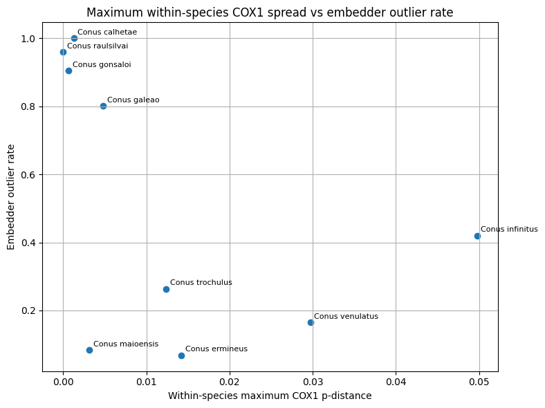
Supplemental figure 6
This figure shows within-species COX1 spread in relation to embedder outlier rate, with point size proportional to the number of COX1 sequences available for each species. By incorporating sequence count directly into the display, the figure helps distinguish patterns supported by broader molecular sampling from those based on sparse representation, providing additional context for interpreting concordance or discordance between mitochondrial variation and embedding-based heterogeneity.
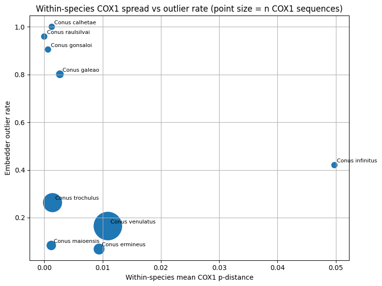
Code and implementation materials
To improve transparency and reproducibility, the implementation materials associated with this study have been archived on Zenodo and are publicly available at DOI: 10.5281/zenodo.19136611. The archive includes four components: MySQL DDL, Python scripts, PHP user-interface code, and training and analysis notebooks. The deposited materials document the benchmark implementation as used within the broader project infrastructure, although they are not intended to function as a standalone software package. Zenodo provides a stable public archive and citable DOI for the deposited materials.