Conservative Statistical Label Curation for Leakage-Aware CNN Species Classification of Harpa Röding, 1798
Published on: July 2026

Abstract
Fine-grained shell classification is sensitive not only to model architecture, but also to label quality, class imbalance, source structure, and validation leakage. This study evaluated whether a fully automatic statistical audit could improve a 13-class CNN species classifier for the gastropod genus Harpa without expert taxonomic redetermination or image relabelling. A leakage-aware EfficientNetV2B2 classifier was trained on an expanded YOLO-transformed dataset containing 17,923 image records, with 14,348 records in the training partition and 3,575 records in a fixed validation partition. Training images were scored out-of-fold, and label-quality evidence was combined with model confidence, prediction margin, entropy, technical preprocessing diagnostics, and embedding-based k-nearest-neighbour support.
Initial curation policies showed that broad statistical filtering can be unsafe in long-tailed fine-grained datasets. A strict policy removed only 128 training images globally, but disproportionately affected rare or difficult species, especially H. kolaceki and H. gracilis. A subsequent pair-aware policy reduced this rare-class erosion by retaining 269 boundary-zone candidates and 81 hard examples while quarantining 86 statistical exclusions and one technical/preprocessing exclusion. Synthetic validation confirmed that random 2% label noise was readily detectable: Cleanlab Top-K recovered 230 of 287 injected errors. Boundary-like species-pair noise was much harder: Cleanlab Top-K recovered 153 of 287 injected errors, and combined Cleanlab, out-of-fold, and kNN evidence recovered only 154.
The final controlled comparison favoured the most conservative exclusion-only policy. This policy quarantined only 25 of 14,348 training images. Relative to the three-run unfiltered baseline cohort, validation accuracy and weighted F1 improved robustly (+0.56 and +0.60 percentage points, each large relative to baseline run-to-run variability), while macro F1 (+1.37 percentage points) and validation loss (−0.0009) moved in the same favourable direction but within the run-to-run variability of the cohort. All four aggregate measures therefore shifted favourably under a single policy, with the accuracy and weighted-F1 gains being the more robust. These descriptive cohort results support a small-removal hypothesis: in fine-grained shell classification, automatic audit is most useful when it removes only extreme, convergent statistical contradictions while retaining boundary-zone and hard-example material. The selected policy should be treated as a candidate policy for the current Harpa dataset version, with continued species-level monitoring, not as a universal taxonomic or curation rule.
Introduction
Image-based species identification has become a practical component of biodiversity informatics, especially when transfer learning and modern convolutional neural networks are used in taxonomically constrained settings. Reviews of automated species recognition emphasize that useful performance is possible, but that model reliability depends not only on architecture, but also on dataset composition, label quality, class balance, and evaluation design [1, 2]. For molluscan shell identification, this is particularly relevant because the visual signal is fine-grained: species may differ by subtle combinations of shell outline, sculpture, colour pattern, aperture structure, varices, wear state, and viewpoint-dependent morphology [3]. EfficientNetV2 is a suitable backbone family for such work because it was designed for efficient fine-tuning and faster training while retaining strong representational capacity [4].
The genus Harpa provides a useful but difficult test case for species-level shell classification. Harpidae is a morphologically distinctive gastropod family within modern gastropod classification, and species-level distinction in Harpa remains largely dependent on shell characters such as shell form, axial ribs or varices, colour pattern, and related conchological features [5, 6]. Recent molluscan and shell-imaging studies show that automated shell classification is feasible in related contexts, including gastropod shell morphology, ark-shell phenotype classification, and visually similar Conus species recognition [7, 8, 9, 10, 11] However, these studies also reinforce a central limitation of biological image classification: high validation accuracy does not by itself prove that the training labels, split strategy, or learned decision boundaries are scientifically reliable.
This issue is especially important for image datasets assembled from online or heterogeneous sources. Species names may be copied between sources, assigned with varying confidence, affected by synonymy or outdated usage, or attached to images that are atypical, damaged, poorly cropped, duplicated, or photographed from unusual viewpoints. In a fine-grained genus such as Harpa, a wrong prediction can therefore have several explanations: a true label error, a difficult but correctly labelled specimen, a weak image, a preprocessing problem, a source-domain effect, or genuine visual overlap between closely related or morphologically similar species. The practical curation problem is not simply to remove every suspicious image, but to separate harmful contradictory supervision from informative hard examples.
Leakage-aware evaluation is a necessary precondition for such a study. Cross-validation and validation-set performance can be optimistically biased when model selection, tuning, and error estimation are not properly separated [12]. In image classification, the same problem appears when related images, near-duplicates, slices, specimens, pages, or acquisition sessions are split across training and validation partitions. Medical and benchmark-imaging studies have shown that such leakage can materially inflate apparent accuracy [13, 14, 15]. For shell images, the equivalent risk is that multiple views or near-duplicate photographs of the same specimen allow a model to learn specimen-specific shortcuts rather than generalizable species-level morphology. The present study therefore treats leakage-aware splitting as part of the scientific design rather than as a secondary implementation detail.
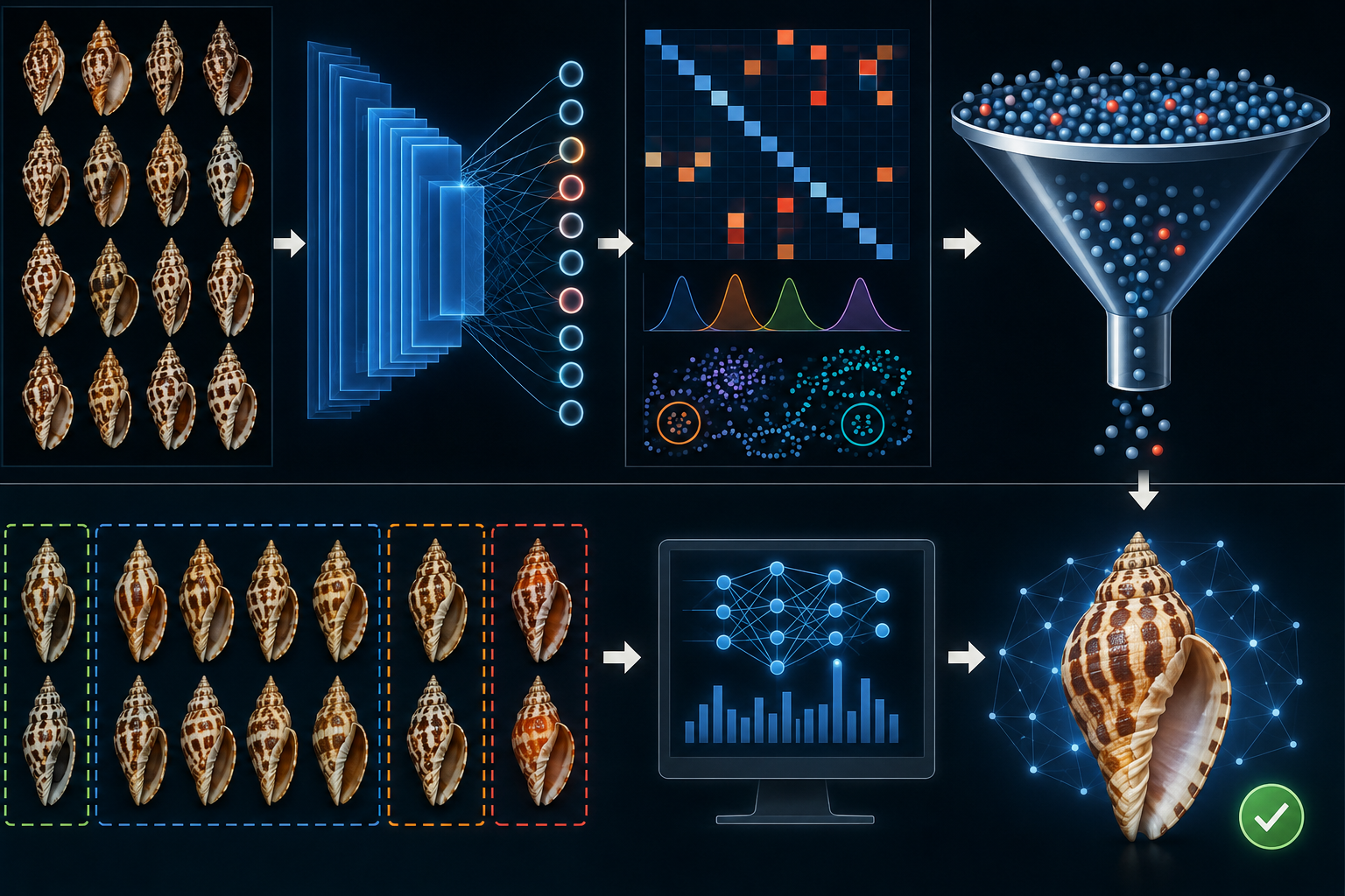
Automated label-quality estimation offers one route to improving such datasets without requiring complete expert redetermination. Confident Learning, implemented in tools such as Cleanlab, uses out-of-sample predicted probabilities to estimate and rank likely label issues [16]. This is well aligned with a shell-classification audit, provided that the probabilities are generated out-of-fold: each training image should be scored by a model that did not train on that same image. Additional evidence can be obtained from prediction confidence, prediction margin, entropy, agreement across repeated seeds, and local feature-space structure. Embedding-based and k-nearest-neighbour methods are useful complements because they ask whether an image is locally supported by neighbours of its assigned species or instead clusters with an alternative species [18, 19].
Nevertheless, the label-noise literature warns against treating automated suspiciousness as proof of mislabelling. Label-cleaning methods are best interpreted as prioritisation or curation tools rather than autonomous taxonomic judges [20, 21]. This caution is particularly important in long-tailed and imbalanced datasets, where rare classes and hard clean samples are more likely to be mistaken for noise [22, 23, 24, 25]. In a species-level Harpa classifier, aggressive pruning could therefore remove exactly the boundary-defining examples needed to learn difficult distinctions, especially for low-support species or recurrent confusion pairs.
The goal of this project is therefore operational dataset curation, not expert taxonomic redetermination. No image is relabelled to another species, and a quarantined record is not claimed to be taxonomically wrong. Instead, the classifier is used as a dataset-audit instrument: images may be excluded from a specific training version only when predefined statistical evidence indicates that they are strongly inconsistent with the intended training signal or outside the intended image scope. The central research question is whether a conservative automatic audit procedure can detect probable harmful label errors in a genus-level Harpa training dataset, and whether excluding only those statistically extreme cases improves or stabilizes species-level classification.
This study evaluates that question in a staged manner. First, a leakage-aware EfficientNetV2B2 baseline is selected for a 13-class Harpa species classifier. Second, several operational curation policies are tested, ranging from strict statistical quarantine to pair-aware hard-example preservation. Third, synthetic label-noise experiments are used as positive controls to distinguish gross random label-error detectability from more realistic boundary-like species-pair ambiguity. Finally, conservative exclusion-only profiles are compared by controlled retraining against the unfiltered baseline. The intended outcome is not a universal rule for all shell datasets, but a reproducible, dataset-version-specific policy for deciding when automatic statistical evidence is strong enough to justify removing a training record.
Methods
Dataset scope and taxonomic classes
The dataset used in this study was defined as a species-level image-classification dataset for the genus Harpa Röding, 1798. The classification task contained 13 operational species classes: Harpa amouretta, H. articularis, H. cabriti, H. costata, H. crenata, H. davidis, H. doris, H. goodwini, H. gracilis, H. harpa, H. kajiyamai, H. kolaceki, and H. major (see Table S1). These classes correspond to the fixed class policy used for the Harpa audit experiments; taxa outside this 13-class policy were not used for model training, out-of-fold scoring, Cleanlab analysis, curation-policy materialization, or downstream retraining.
The final expanded leakage-aware dataset contained 17,923 image records: 14,348 records in the training partition and 3,575 records in the validation partition.
Each image record was associated with an accepted Harpa species name. Where source names required harmonization, labels were normalized to the accepted names used in the 13-class policy. These labels were treated as dataset labels for model training and audit analysis, not as new taxonomic determinations made by this study; the audit workflow did not relabel records, infer synonymy, split species, or merge species.
Species-level image support was strongly imbalanced in the full 17,923-record dataset. The largest classes were H. harpa (3,832 images), H. major (3,659 images), and H. articularis (2,506 images), whereas the smallest classes were H. gracilis (85 images), H. kolaceki (106 images), and H. goodwini (128 images). Training-partition counts were lower and are reported separately in the curation-policy tables.
Image preprocessing and YOLO-based shell extraction
Some calibration conditions used original source images, whereas others used YOLO-transformed shell-instance crops. The YOLO preprocessing pipeline converted heterogeneous shell photographs into object-centred classifier inputs by detecting the shell, extracting the shell region, standardizing the background, and recording preprocessing diagnostics.
The preprocessing pipeline followed the same general design as the YOLO-based pipeline used in the earlier Morum study [27]. A custom Ultralytics YOLO shell-segmentation model was applied to raw source images to detect shell instances and produce bounding boxes and segmentation masks. This object-centred preprocessing is consistent with fine-grained visual-classification work in which object localization functions as an attention mechanism, reducing irrelevant image regions and increasing the relative prominence of diagnostic morphology [28, 29]. In mollusk-image classification, YOLO-style localization has also been used in shell-related CNN workflows, and earlier IdentifyShell work found YOLO-assisted object-centric preprocessing useful for operational shell-image classification [30, 27].
The transformed classifier image was generated from the selected shell instance. The non-zero segmentation-mask region defined the object crop, and the crop was padded around the shell so that the specimen was not cut too tightly. Crop coordinates were clipped at the original image boundaries where necessary. The RGB pixels belonging to the shell mask were then pasted onto a black background. The resulting shell crop was placed on a square black canvas, producing a standardized object-centred image. This procedure reduced framing and background variation, but it was treated as a controlled design choice rather than as an automatically superior representation, because CNNs may exploit background or source-specific image context as shortcut information [31, 32].
When a source image contained multiple detected shell instances, the preprocessing pipeline could generate separate instance-level transformed outputs, distinguished by detection index or output filename. In the downstream Harpa training manifests, each transformed image was treated as one classifier input. If no usable shell detection, segmentation mask, or crop could be derived, the source image did not contribute a normal transformed training crop. Such cases were recorded in the preprocessing metadata when available and could later appear as technical-warning evidence rather than as ordinary label-audit candidates.
Technical diagnostics included detection confidence, detection count, crop geometry, mask geometry, crop-boundary contact, shell-size flags, detection-failure flags, multi-detection flags, warning severity, and warning reason. These diagnostics were evaluated before statistical label-audit evidence, so that image/preprocessing failures were separated from possible label inconsistencies.
YOLO warnings were not interpreted as proof of taxonomic mislabelling. They were used to separate possible image/preprocessing failures from statistical label-inconsistency evidence. Conversely, the absence of a strong preprocessing warning did not rule out a statistical label contradiction.
Because YOLO transformation, dataset expansion, and split policy changed together in several calibration conditions, these comparisons were treated as dataset-construction conditions rather than as a clean causal ablation of YOLO preprocessing alone.
Leakage-aware train-validation splitting
The train-validation split was grouped so that known related images, repeated specimen views, transformed outputs, and images derived from the same source record were assigned to the same partition rather than split independently. This reduced the risk of validation leakage from near-duplicate or specimen-linked images [12, 13, 14, 15 ].
The Harpa leakage-aware dataset was generated as a predefined train-validation folder structure before the
audit experiments. The split used a fixed split seed of 20260606 and a target validation
ratio of 20%. In the final expanded leakage-aware YOLO-transformed dataset, 17,923 image records were
retained: 14,348 records in the training partition and 3,575 records in the validation partition. This
corresponds to an achieved validation ratio of 19.95%. These counts define the fixed dataset substrate
used for the downstream audit-impact comparisons.
Related images were assigned to a shared split group before partitioning. The grouping priority followed the Morum leakage-aware workflow [27]: use the strongest available specimen-, listing-, source-page-, source-URL-, base-image-, shell-record-, transformed-image-, or hash-based identifier, and use a filename fallback only when no stronger identifier was available. All images sharing the selected group identifier were assigned as a unit to either training or validation.
The split was species-aware in the sense that the 13 operational Harpa classes were preserved in both partitions wherever the available image counts allowed this. However, the grouping rule took precedence over independent image-level randomization: images were not split one-by-one if they belonged to the same preferred group. This means that the achieved validation ratio could deviate slightly from exactly 20%, but the resulting validation partition was more appropriate for estimating generalization to independent image groups.
Audit decisions were applied only to the 14,348-image training partition; the 3,575-image validation partition was kept fixed for downstream comparison.
The downstream audit baseline was selected from the expanded leakage-aware YOLO condition, not from the highest-scoring normal-split condition, because audit impact had to be evaluated against the grouped validation design.
The same leakage-aware training partition also served as the source population for out-of-fold label-audit evidence. Out-of-fold prediction generation was performed only inside the 14,348-image training partition, while the external 3,575-image validation partition remained untouched for final model evaluation. This separation was necessary because label-audit evidence should be generated from predictions made on images that were not used to train the scoring model, while downstream training impact should be evaluated on a stable validation set.
CNN architecture and training protocol
All pre-audit Harpa calibration experiments used the same general IdentifyShell EfficientNetV2-based image-classification framework. The classifier backbone was EfficientNetV2B2 initialized with ImageNet pretrained weights and adapted to the 13-class Harpa species task by replacing the original ImageNet classification head with a genus-specific softmax classification head [4]. This architecture was used because EfficientNetV2 was designed for efficient fine-tuning and strong image-recognition performance at moderate computational cost.
Input images were loaded as RGB images and resized to 400 × 400 pixels before being passed to the network. Depending on the experimental condition, these inputs were either original source images or YOLO-transformed shell-instance crops. The model head followed the same general design as the earlier Morum classifier: the EfficientNetV2B2 convolutional backbone was followed by global average pooling, batch normalization, dropout, and a dense species-classification layer. The final dense layer produced 13 softmax probabilities, one for each operational Harpa species class.
Training used transfer learning rather than training the convolutional backbone from scratch. The EfficientNetV2B2 backbone was initialized from ImageNet weights, after which partial fine-tuning was performed within the existing IdentifyShell training framework. Following the framework used in the Morum study, the backbone was initially treated as a pretrained feature extractor and later fine-tuned by unfreezing the final backbone layers, while batch-normalization layers in the fine-tuned region were kept frozen. This strategy was intended to adapt high-level visual features to shell morphology while limiting instability in a moderate-sized biological image dataset.
Models were trained with Adam [33], batch size 64, and a maximum of 100 epochs. The default learning rate was 0.0005, with one calibration condition using 0.0004 together with higher classifier-head dropout. Early stopping monitored validation loss and restored the best validation-loss weights.
The calibration series compared class-weighted categorical cross-entropy, class-balanced sampling, and focal loss. Class-balanced sampling oversampled minority classes with replacement, increasing training exposure from 11,132 natural files to 30,459 sampled paths in that condition without creating new image files. Focal-loss conditions used alpha = 0.25 and gamma = 2.0 [34]. Later focal-loss conditions added regularization of 0.001 and classifier-head dropout of 0.3 or 0.4.
No separate runtime image-augmentation experiment was used as an independent factor in the pre-audit comparison. The main image-representation changes in Table 1 were dataset construction changes: no YOLO preprocessing, normal YOLO-transformed data, leakage-aware YOLO-transformed data, and expanded YOLO-transformed data. Validation images were not augmented, resampled, class-balanced, or relabelled. This was necessary so that differences between runs could be interpreted against a stable validation set.
| Component | Setting used in this study |
|---|---|
| Backbone | EfficientNetV2B2 |
| Initialization | ImageNet pretrained weights |
| Input size | 400 × 400 RGB |
| Classification head | Global average pooling, batch normalization, dropout, dense 13-class softmax layer |
| Optimizer | Adam |
| Learning rate | 0.0005 by default; 0.0004 in the lower-learning-rate calibration condition |
| Batch size | 64 |
| Maximum epochs | 100, with early stopping |
| Early stopping | Validation-loss monitoring with best-weight restoration |
| Class weights | Used in early class-weighted conditions and one focal-loss condition |
| Class-balanced sampling | One calibration condition; 30,459 sampled paths from 11,132 natural files |
| Focal loss | Alpha = 0.25, gamma = 2.0 |
| Regularization | 0.001 in later focal-loss conditions |
| Top dropout | 0.3 or 0.4 in later focal-loss conditions |
Baseline cohort for downstream audit comparison
The downstream audit comparisons used a three-run unfiltered baseline cohort rather than a single pre-audit
calibration run. This distinction is important because Runs 10 and 11 were calibration conditions used
to identify the expanded leakage-aware YOLO dataset condition as the appropriate audit-compatible baseline
family. The final downstream comparison, however, was made against a separate three-run baseline cohort
defined in the audit-comparison artifacts as Run 10, Run 15, and
Run 16.
All three baseline-cohort runs were treated as uncurated reference runs. No Curation Policy 3 quarantine, Cleanlab exclusion, k-nearest-neighbour exclusion, hard-example protection, or boundary-zone decision was applied to the training set before these baseline models were trained. The cohort therefore represented the model behaviour expected from the selected expanded leakage-aware YOLO dataset condition before any label-audit intervention.
The baseline cohort was used to reduce dependence on a single stochastic training outcome. This follows the same reporting principle used in the Morum study, where model families were compared across repeated controlled seeds rather than selected from a single favourable run [27]. In the Harpa audit comparison, the baseline cohort provided the reference distribution against which single-run curation ablations and three-run final policy retraining results were evaluated.
For each baseline run, validation accuracy, macro F1, weighted F1, and validation loss were extracted from the corresponding training and evaluation artifacts. The three-run cohort provided the unfiltered reference distribution for downstream audit comparisons; means and standard deviations were computed as defined in the Evaluation metrics and statistical reporting subsection.
Out-of-fold prediction and label-quality evidence
Out-of-fold (OOF) prediction was used to generate label-audit evidence for the training partition without allowing an image to be scored by a model that had trained on that same image. This was required because the audit workflow used model disagreement, confidence, prediction margin, entropy, and later Cleanlab label-quality evidence as statistical signals. In-sample predictions would risk self-confirming memorization, especially in a fine-grained shell dataset with repeated visual structure. OOF prediction therefore served as an evidential safeguard: each training image received a probability vector from a model for which that image was held out from fitting. This follows the confident-learning requirement that label-quality estimation should use out-of-sample predicted probabilities [16].
The OOF procedure was applied only inside the leakage-aware training partition. The external leakage-aware validation partition remained untouched and was reserved for downstream baseline-versus-curated model evaluation. Thus, there were three distinct validation concepts in the workflow: the fixed external validation set for final model comparison, the internal per-fold validation set used during fold-model training, and the per-fold OOF holdout set used only for audit prediction. The OOF holdout images were not used for model fitting or early stopping in their corresponding fold model.
Each OOF fold contained a fold-training subset, an internal validation subset, and an OOF holdout subset. One fold-specific EfficientNetV2B2 classifier was trained per fold, then applied only to that fold’s OOF holdout images. Across the three folds, this produced one out-of-sample prediction for each of the 14,348 training images.
The fold-generation validation checks confirmed that all groups were assigned to a valid OOF fold, all species were present in each OOF holdout, all species were present in each fold-training subset, all species were present in each internal fold-validation subset, and the combined OOF rows reconciled to 14,348 records. These checks were important because the OOF evidence was later used for image-level curation decisions; missing species or unreconciled rows would have made the label-audit evidence incomplete.
After all three fold models had been trained and their OOF holdouts had been scored, the fold-level outputs were concatenated into Cleanlab-ready combined artifacts.
OOF prediction evidence was treated as statistical audit evidence. It was not used alone for relabelling or quarantine; it provided the probability substrate for Cleanlab and one component of the combined evidence used by later curation policies.
Cleanlab / confident-learning evidence
Cleanlab evidence was derived from the out-of-fold probability matrix produced for the training partition. The input to the confident-learning step consisted of one row per training image, with a 13-class probability vector from the out-of-fold classifier and the corresponding observed dataset label encoded as an integer class. The probability vector represented the model’s out-of-sample belief over the 13 operational Harpa species classes, whereas the observed label represented the species name assigned in the dataset after taxonomic normalization. The method therefore compared what the out-of-fold model predicted with the label used for training, without using the external validation partition.
Cleanlab was used as a statistical label-quality estimator based on confident learning [16]. For each training image, the method produced a label-quality score and an issue ranking. Lower label-quality scores indicated stronger statistical evidence that the observed label was inconsistent with the out-of-fold probability distribution. In practical terms, a record became more suspicious when the assigned class received low model support and an alternative class received stronger support. The resulting ranking was used as an ordered list of candidate label issues, not as an automatic list of confirmed mistakes.
The Cleanlab output was joined back to the row-level audit table so that label-quality evidence could be interpreted alongside the out-of-fold top prediction, prediction confidence, prediction margin, entropy, source metadata, technical preprocessing diagnostics, and later embedding-neighbourhood evidence. Cleanlab was therefore not used as a standalone relabelling system. It supplied one evidence stream within a broader curation workflow.
Candidate ranking was interpreted conservatively. The highest-ranked candidates were records for which the observed dataset label and the out-of-fold probability evidence were most inconsistent. However, a high Cleanlab rank did not establish that the taxonomic label was wrong. In a fine-grained shell dataset, the same signal may arise from an actual label error, a difficult but correctly labelled shell, an unusual viewpoint, poor image quality, preprocessing failure, source-domain shift, or genuine species-pair ambiguity. For this reason, Cleanlab candidates were described as statistical label-issue candidates rather than confirmed taxonomic errors, consistent with the broader label-cleaning literature [20, 21].
When a fixed-size ranked subset was required, candidates were selected from the top of the Cleanlab ranking. In real Harpa data, this ranking was used only as statistical prioritisation because no ground-truth list of true label errors was available.
Cleanlab evidence could support quarantine only when combined with additional criteria defined by a curation policy. The workflow did not relabel images to a suggested alternative class, did not treat every ranked candidate as wrong, and did not use Cleanlab alone to define the final audited training set.
Embedding and k-nearest-neighbour evidence
Embedding evidence was used as a local-structure check on OOF prediction and Cleanlab evidence. It asked whether an image was locally supported by neighbours of its assigned species or instead embedded closer to the classifier-predicted species. This evidence was treated as corroboration only, consistent with noisy-label work showing both the usefulness and risks of feature-neighbourhood methods [18, 19, 21, 25 ].
Embeddings were extracted from the same out-of-fold classifier framework used for audit prediction. Each image was embedded by the fold-specific classifier for which that image belonged to the held-out fold, so the embedding was generated without training the model on that same image. The Harpa evidence report documents a 1,408-dimensional CNN feature vector for each of the 14,348 training images. These vectors represented the learned visual feature representation before conversion into the final 13-class species probability output, rather than the softmax probabilities themselves.
Nearest-neighbour evidence was computed in this 1,408-dimensional embedding space using cosine distance. For each image, the procedure searched the embedding matrix for its nearest neighbours and excluded the query image itself from its own neighbourhood. The primary neighbourhood size was K = 20. If the image itself appeared among the returned neighbours, it was removed and the next closest image was retained so that each record was evaluated against 20 distinct neighbouring records.
For each image, the neighbourhood labels were summarized in three ways. First, the assigned-label support was calculated as the fraction of the 20 neighbours whose dataset label matched the image’s assigned species. Second, the predicted-label support was calculated as the fraction of the 20 neighbours whose dataset label matched the classifier’s top-1 predicted species. Third, the dominant neighbourhood label was recorded as the species label occurring most frequently among the neighbours. When two or more labels were tied for dominance, the label with the smallest mean neighbour distance was selected as the dominant neighbourhood label.
The interpretation was directional. High assigned-label support indicated that the image was embedded among visually similar records carrying the same dataset label. High predicted-label support, especially when the out-of-fold classifier also disagreed with the assigned label, indicated that the image was embedded closer to the model-predicted species than to its assigned species. Low support for both assigned and predicted labels indicated a less coherent or more ambiguous local neighbourhood rather than a direct label-error conclusion.
Species-centroid distances were also computed from the same embedding matrix. For each of the 13 species, a centroid was calculated as the mean embedding of all records assigned to that species. Under the cosine-distance setting, centroids were normalized before distance comparisons. Each image was then compared with all species centroids, allowing the workflow to record whether the assigned species centroid or the predicted species centroid was closer in embedding space. These centroid distances were used as supporting context alongside the K-nearest-neighbour rates.
Embedding contradiction evidence was defined only when several conditions converged. A record was considered more suspicious when it had low neighbourhood support for its assigned label, higher support for the model-predicted label, disagreement between assigned and predicted species, and centroid evidence favouring the predicted species over the assigned species. Conversely, an image with strong assigned-label neighbourhood support was treated as locally supported, even if other statistical signals marked it as difficult. This distinction was important for rare or boundary-like species, where unusual but valid examples may appear statistically suspicious.
Neighbourhood evidence was not used for relabelling. It served as a confirmation signal for exclusion-only policies when it converged with OOF prediction and label-quality evidence.
Curation-policy definitions
Curation policies were defined as training-set decision rules applied to the 14,348-image training partition. The policies did not relabel images, did not create new taxonomic determinations, and did not modify the fixed 3,575-image validation partition. Each policy assigned a training action to a record: retain it for training, retain it with a special hard-example or boundary-zone designation, or quarantine it from a specific exported training set. A quarantine decision therefore meant that a record was considered operationally unsafe for that training version, not that the shell was confirmed to be taxonomically misidentified.
The policies were ordered from broad statistical filtering toward increasingly conservative exclusion. Early policies tested strict statistical quarantine and hard-example protection. The pair-aware policy added automatic boundary-zone retention and safeguards. The final strict policies disabled boundary-zone detection and tested exclusion-only rules based on convergent Cleanlab, OOF, and neighbourhood evidence.
The shared evidence sources were the out-of-fold model prediction, top-1 confidence, prediction margin, entropy, Cleanlab label-quality evidence, technical/preprocessing diagnostics, and, for policies that used it, embedding-based k-nearest-neighbour support. Cleanlab evidence was used as a statistical label-quality signal [16]. Embedding and k-nearest-neighbour evidence were used as local visual-neighbourhood corroboration rather than as an independent relabelling mechanism [18, 19 ].
Decision semantics
The curation policies used five operational decision types. Ordinary retention meant that the image remained in the training set without special designation. Hard-example retention meant that the image was suspicious or difficult, but was deliberately kept because removing it risked eroding useful species-boundary information. Boundary-zone retention meant that the image belonged to a recurrent species-pair conflict pattern and was retained as potentially informative ambiguous material. Statistical quarantine meant that the image was removed from the exported training set because the statistical evidence indicated a strong contradiction with the assigned species label. Technical quarantine meant that the image was removed because image extraction or preprocessing evidence indicated an operational image/preprocessing failure.
Curation Policy 1: strict statistical quarantine
Curation Policy 1 was a strict exclusion policy based on statistical label-inconsistency evidence. Boundary-zone detection was disabled, protected hard examples were not allowed, and the policy was not pair-aware. Records either remained in training or were quarantined as statistical exclusions.
Curation Policy 2: strict quarantine plus manually protected hard examples
Curation Policy 2 was an exploratory safeguard policy, not the final automatic audit policy. It used the same strict statistical quarantine rule as Curation Policy 1 but retained a small set of manually protected hard examples that would otherwise have been quarantined. Boundary-zone detection was not active as an automatic detector. The policy was included to test whether protecting high-risk boundary-like examples could reduce rare-class erosion; it was not used as the final scalable curation rule.
Curation Policy 3 medium: automatic pair-aware curation
Curation Policy 3 medium replaced manual hard-example protection with an automatic pair-aware profile. Boundary-zone detection was active. Protected hard examples were allowed, but protection was assigned by predefined automatic safeguards rather than by manual image-level selection. The policy combined image-level, species-level, pair-level, and technical evidence before assigning a training action.
At image level, the policy used out-of-fold prediction disagreement, prediction confidence, prediction margin, entropy, Cleanlab label-quality evidence, neighbourhood support for the assigned label and predicted label, and technical/preprocessing diagnostics. Species-level safeguards limited excessive removal from low-support or weak classes. Pair-level safeguards identified recurrent assigned-species to predicted-species conflicts, reciprocal confusion patterns, embedding overlap, and source or technical context. The policy therefore treated recurrent pair-level conflict differently from isolated high-confidence contradiction.
The policy produced five possible outcomes: ordinary retention, boundary-zone retention, hard-example retention, statistical quarantine, and technical quarantine. Boundary-zone and hard-example records remained in the exported training set. Statistical and technical quarantine records were excluded from the exported training set. This design made CP 3 medium more conservative than CP 1 and CP 2 in recurrent boundary-like regions, while still allowing strong isolated contradictions to be removed.
Technical diagnostics were evaluated before statistical label-inconsistency decisions. This ordering prevented image/preprocessing failures from being misinterpreted as taxonomic label contradictions. A technical failure could therefore lead to technical quarantine even when the statistical label-evidence pathway was not used.
Strict Cleanlab+OOF final ablation policy
The Strict Cleanlab+OOF policy was an exclusion-only final ablation. It used Cleanlab label-quality evidence together with out-of-fold model-confidence contradiction. Boundary-zone detection was disabled, and protected hard examples were not allowed. The policy therefore produced only two training actions: retain the record or quarantine it as a statistical exclusion.
This policy tested whether a strict combination of label-quality evidence and out-of-fold classifier contradiction was sufficient for conservative curation without using local embedding-neighbourhood confirmation. It was used as an ablation to separate the contribution of Cleanlab+OOF evidence from the additional contribution of k-nearest neighbours.
Strict Cleanlab+OOF+KNN final ablation policy
The Strict Cleanlab+OOF+KNN policy extended the previous strict ablation by requiring k-nearest-neighbour confirmation. Boundary-zone detection was disabled, and protected hard examples were not allowed. The policy remained exclusion-only: records were either retained or quarantined.
The purpose of this policy was to test whether local embedding-neighbourhood evidence improved the reliability of strict statistical exclusion. A record was more likely to qualify for quarantine when Cleanlab evidence, out-of-fold model contradiction, and neighbourhood support all pointed away from the assigned label and toward the predicted alternative. Neighbourhood evidence was therefore used as confirmation, not as a standalone rule.
Very Strict Cleanlab+OOF+KNN final selected policy
The Very Strict Cleanlab+OOF+KNN policy was the final conservative exclusion-only profile. It used the same evidence family as Strict Cleanlab+OOF+KNN, but applied the most conservative decision rule. Boundary-zone detection was disabled, protected hard examples were not allowed, and the policy produced only retention or quarantine decisions.
This policy was designed to remove only extreme, convergent statistical contradictions. A record required simultaneous support from very low label-quality evidence, strong out-of-fold prediction contradiction, high prediction confidence and margin, strong neighbourhood support for the predicted alternative, and weak neighbourhood support for the assigned label. Recurrent boundary-like species-pair conflicts were not removed merely because they were difficult; they could be quarantined only if they also satisfied the very-strict contradiction criteria.
| Policy | Boundary-zone detection | Protected hard examples | kNN confirmation | Species / pair safeguards | Decision outputs |
|---|---|---|---|---|---|
| Curation Policy 1: strict statistical quarantine | Disabled | Not allowed | Not required | Not pair-aware | Retention or statistical quarantine |
| Curation Policy 2: strict quarantine plus protected hard examples | Disabled as an automatic detector | Allowed by manual protection | Not required | Manual protection of selected high-risk cases | Retention, protected hard-example retention, or statistical quarantine |
| Curation Policy 3 medium: automatic pair-aware profile | Active | Allowed automatically | Used in combined evidence | Active species caps and pair safeguards | Retention, boundary-zone retention, hard-example retention, statistical quarantine, or technical quarantine |
| Strict Cleanlab+OOF | Disabled | Not allowed | Not used | Boundary handling disabled | Retention or statistical quarantine |
| Strict Cleanlab+OOF+KNN | Disabled | Not allowed | Required | Boundary handling disabled | Retention or statistical quarantine |
| Very Strict Cleanlab+OOF+KNN | Disabled | Not allowed | Required | Boundary-like cases excluded only if they met the very-strict contradiction rule | Retention, statistical quarantine, or technical quarantine |
The distinction between pair-aware retention and exclusion-only filtering is central to the method. CP 3 medium allowed the audit workflow to document ambiguous or recurrent species-pair cases without removing them from training. The final strict profiles intentionally disabled that boundary-zone branch because their purpose was different: to test whether only the strongest statistical contradictions should be removed. Thus, boundary-zone material was treated as useful training signal unless it also satisfied the very-strict exclusion criteria.
Synthetic label-noise validation experiments
Synthetic label-noise experiments were used as positive-control tests for the audit pipeline. The real Harpa training set did not contain an independently verified list of true label errors, so precision and recall could not be measured directly on real audit candidates. To create an evaluable test condition, a known subset of training labels was deliberately changed before running the same out-of-fold and Cleanlab-based detection procedure. The injected labels were hidden from the detection pipeline and were used only after ranking to score recovery performance. This design follows the general noisy-label evaluation logic that known perturbations can be used to test whether a label-quality method can recover controlled errors [16, 26].
Both synthetic experiments used the same fixed dataset substrate as the audit workflow: 17,923 total image records, consisting of 14,348 training records and 3,575 validation records. Label injection was applied only to the training partition. The validation partition was not changed, relabelled, or used to define injected errors. The injected-error rate was 2% of the training partition, giving 287 hidden injected label changes. Therefore, the primary ranked evaluation used K = 287.
The primary detection endpoint was Cleanlab Top-K recovery. After label injection, candidates were ranked using the same OOF/Cleanlab evidence pipeline as the real audit workflow. The top 287 records were then compared with the hidden injected-error list.
The first experiment used random 2% label injection. In this positive-control condition, 287 training labels were changed to incorrect labels without constraining the replacement label to a visually plausible neighbouring species. This created strong artificial label contradictions. The purpose was to test whether the OOF/Cleanlab pipeline could recover gross label errors when the injected label was arbitrary rather than biologically or visually plausible.
The second experiment used boundary-like 2% label injection. In this harder condition, replacement labels were assigned along predefined species-pair routes intended to approximate plausible Harpa confusion structure. The routes are shown in Figure 3.
The boundary-like experiment was designed to test a more realistic failure mode than arbitrary random relabelling. If an injected alternative species is visually close to the original species, the resulting record may resemble a difficult boundary case rather than an obvious label contradiction. This distinction was important because the real audit policy was not intended to remove every ambiguous species-pair example. It was intended to remove only records with strong statistical evidence of harmful contradictory supervision.
A third analysis used the same boundary-like injected labels but ranked candidates using combined evidence rather than Cleanlab alone. This combined ranking used Cleanlab label-quality evidence together with out-of-fold model-confidence contradiction and embedding/k-nearest-neighbour support. The objective was to test whether adding confidence and neighbourhood evidence improved boundary-like Top-K recovery over the Cleanlab-only ranking. The same K = 287 evaluation was used so that the Cleanlab-only and combined rankings could be compared directly.
For each synthetic evaluation, records selected in the Top-K set were counted as true positives if they belonged to the hidden injected-error list and as false positives if they did not. Injected records not selected in the Top-K set were counted as false negatives. Precision, recall, and F1 were then calculated from these counts. For the boundary-like experiment, recovery was also summarized by species-pair route so that failures could be separated into easy-to-detect and difficult-to-detect boundary pairs.
Synthetic recovery was interpreted as a diagnostic property of the audit evidence, not as a direct estimate of the number of true errors in the real Harpa dataset. Strong recovery in the random-injection condition indicated that the pipeline could detect gross artificial contradictions. Weaker recovery in the boundary-like condition indicated that plausible species-pair ambiguity was harder to separate from genuine hard examples. This distinction justified conservative downstream curation: statistical evidence may support exclusion of strong contradictions, but boundary-like cases require additional caution [20, 21, 25].
Retraining after curation
After each curation policy assigned training-set decisions, a policy-specific export converted those decisions into training, validation, and quarantine manifests. Ordinary retained records, hard examples, and boundary-zone candidates were included in the exported training manifest. Statistical and technical quarantine records were excluded from the exported training manifest and recorded separately for audit traceability.
Quarantine operated through training-set exclusion, not through relabelling. Curated dataset versions were exported separately from the original leakage-aware dataset so that each retraining experiment could be traced to a specific curation policy.
The validation partition was kept unchanged for all retraining experiments. No validation image was removed, relabelled, resampled, or replaced after curation. This was essential because the purpose of retraining was to measure the downstream effect of changing the training set only. The validation manifest therefore remained the same fixed benchmark used for the unfiltered baseline cohort and for all post-curation comparisons.
Retraining used the same 13-class task and EfficientNetV2B2 framework. Audit evidence was used only to construct the exported training manifest; Cleanlab scores, OOF predictions, kNN evidence, boundary-zone flags, and quarantine reasons were not provided as model inputs during retraining.
For each retrained model, validation metrics were extracted from the completed training and evaluation artifacts. These metrics were later compared with the unfiltered baseline cohort using the reporting rules defined in the evaluation subsection. Single-run retraining results were treated as directional evidence only, whereas three-run policy cohorts were summarized as mean ± standard deviation. This distinction prevented a single curated run from being overinterpreted as a stable policy effect.
This retraining design made the curation intervention explicit: the classifier architecture, species scope, and validation benchmark were held constant, while the exported training manifest changed according to the selected policy. As a result, any downstream difference between the unfiltered baseline and a curated model was interpreted as the effect of the training-set intervention rather than as a consequence of changing the validation set or redefining the taxonomic task.
Evaluation metrics and statistical reporting
Model performance was evaluated on the fixed leakage-aware validation partition. The primary aggregate classification metrics were validation accuracy, validation loss, weighted F1, and macro F1. Validation accuracy was defined as the number of correctly classified validation images divided by the total number of validation images. Validation loss was the scalar loss value reported on the validation partition by the training/evaluation artifact for the corresponding run. Because the calibration series included different loss configurations, validation loss was interpreted most directly within comparable retraining conditions and was not used alone as a cross-condition selection criterion.
Precision, recall, and F1 were calculated from the validation-set confusion matrix. For a given species, precision was defined as true positives divided by all images predicted as that species. Recall was defined as true positives divided by all validation images assigned to that species. Species-level F1 was the harmonic mean of species-level precision and recall:
F1 = 2 × precision × recall / (precision + recall)
Per-species recall and per-species F1 were used to identify weak classes that could be hidden by high global accuracy. This was important because the Harpa dataset was imbalanced, and a model could perform well on large classes while remaining unreliable for rare or visually difficult species.
Weighted F1 was defined as the mean of the per-species F1 scores weighted by the number of validation images belonging to each species. This metric therefore reflects the class distribution of the validation set and gives larger classes more influence. Macro F1 was defined as the unweighted mean of the per-species F1 scores, giving each species equal weight regardless of its validation-set size. Macro F1 was therefore treated as the more sensitive aggregate measure for rare-species degradation.
Reported macro F1 refers to the macro F1 value stored in the training or evaluation artifact. When per-species F1 values were available, a recomputed macro F1 was calculated as the arithmetic mean of the 13 species-level F1 scores:
recomputed macro F1 = Σ F1species / 13
The recomputed value was used only where the required per-species F1 values were available. Otherwise, the artifact-reported macro F1 was retained and identified as reported macro F1.
Confusion-pair counts were used to summarize recurrent species-pair errors. A confusion-pair count was calculated from the validation predictions by counting assignments between two species in either direction. These counts were used descriptively to identify persistent pair-level failure modes, such as reciprocal or recurrent confusion between visually similar classes. They were not treated as independent statistical tests and were not used as direct evidence of taxonomic error.
Synthetic label-noise detection was evaluated separately from ordinary validation classification. In the synthetic experiments, the ground-truth error set was the hidden list of injected label changes. A flagged record was counted as a true positive if it was one of the injected errors. A flagged record was counted as a false positive if it was selected by the detection rule but was not one of the injected errors. An injected record was counted as a false negative if it was not selected by the detection rule.
Synthetic detection precision was defined as true positives divided by all flagged records:
precision = TP / (TP + FP)
Synthetic detection recall was defined as true positives divided by all injected errors:
recall = TP / (TP + FN)
Synthetic detection F1 was the harmonic mean of synthetic precision and recall:
F1 = 2 × precision × recall / (precision + recall)
For Top-K synthetic evaluation, K was set equal to the number of hidden injected errors. Under this design, the number of flagged records equalled the number of injected records. Therefore, Top-K precision and Top-K recall were numerically identical, although they still represent different quantities: precision measures the purity of the selected Top-K list, whereas recall measures the fraction of injected errors recovered by that list.
Statistical reporting distinguished single-run directional results from repeated-run cohort results. Single-run curation policies were reported as individual outcomes without standard deviation and were interpreted as directional evidence only. They were used to assess whether a policy was promising, harmful, or operationally unsafe, but not to claim a stable final effect.
Cohort results were based on three repeated runs under the same comparison condition. For each metric, the cohort mean was calculated as the arithmetic mean across the three runs:
mean = (x1 + x2 + x3) / 3
Run-to-run variability was reported as the sample standard deviation, using n − 1 in the
denominator:
SD = sqrt(Σ(xi − mean)2 / (n − 1)), with n = 3
Three-run cohort values were therefore reported as mean ± standard deviation. Differences between a curated policy and the baseline cohort were reported in percentage points for accuracy and F1 metrics, and as absolute loss differences for validation loss. This reporting convention followed the same controlled comparison logic used in the preceding Morum study: policy conclusions should be based on repeated controlled runs where available, while single-run ablations should remain explicitly directional rather than conclusive [27].
Software and hardware environment
Model training, out-of-fold prediction, embedding extraction, synthetic label-noise experiments, and post-curation retraining were executed in the project’s GPU-based Python machine-learning environment. The classifier implementation used TensorFlow/Keras with an EfficientNetV2B2 backbone initialized from ImageNet weights. YOLO preprocessing used Ultralytics YOLO, and Cleanlab was used for confident-learning label-quality scoring from OOF predicted probabilities.
| Environment component | Reported value | Reproducibility role |
|---|---|---|
| Training Python | Python 3.10.12 on GPU server / WSL2 | Training, OOF prediction, embedding extraction, synthetic experiments, and retraining. |
| Training TensorFlow / Keras | TensorFlow 2.16.1; standalone Keras 3.3.2 on GPU server | EfficientNetV2B2 model construction, training, validation, and retraining. |
| Cleanlab | Cleanlab 2.9.0 | Label-quality scoring and candidate issue ranking. |
| Ultralytics YOLO | Ultralytics 8.4.41 on GPU server | Shell detection/segmentation and object-centred preprocessing. |
| CUDA / cuDNN | CUDA 12.3; cuDNN 8 on GPU server | GPU acceleration for TensorFlow/Keras and YOLO-related processing. |
| GPU hardware | HP Omen 30L GT13; Intel Core i9-10850K; 64 GB RAM; NVIDIA GeForce RTX 3080 | Training, OOF inference, embedding extraction, and retraining. |
| Reporting / decision storage | MariaDB 10.11.13 | Storage and presentation of audit evidence, decisions, manifests, and summaries. |
Reproducibility artifacts
Reproducibility depended on preserving the dataset manifests and the row-aligned audit evidence used to generate curation decisions. For each dataset version, the retained-training manifest, validation manifest, quarantine manifest, audit decision table, export summary, and retraining metrics were retained.
For label-audit evidence, the required artifacts were the OOF prediction table, predicted-probability matrix, observed-label vector, class mapping, Cleanlab label-quality scores, embedding matrix, k-nearest-neighbour evidence, and policy-specific decision records. These artifacts define which records were scored, retained, quarantined, or evaluated, and are therefore part of the method rather than only reporting output.
Results
Pre-audit model calibration and selection of a leakage-aware baseline
Before evaluating label-audit strategies, a sequence of pre-audit calibration experiments was performed to establish an appropriate baseline for downstream comparison. The purpose of these experiments was not simply to maximize validation accuracy, but to identify a stable and methodologically conservative reference model trained under conditions compatible with later audit experiments. All runs used a 13-class Harpa species classification setting and an EfficientNetV2B2 image-classification backbone with ImageNet transfer learning. The experiments varied dataset construction, leakage-aware splitting, YOLO-based preprocessing, class-balancing strategy, focal loss, regularization, dropout, and learning rate.
The initial reference model (Run 1), used an older Harpa dataset without YOLO preprocessing. It achieved 90.49% validation accuracy, 90.82% weighted F1, and 86.3% macro F1. This indicated that the model was already strong at the aggregate level, but that performance was uneven across species. The lower macro F1, compared with weighted F1, showed that minority or visually difficult classes had a disproportionate effect on the evaluation. At class level, the weakest validation results were concentrated in H. kolaceki, H. davidis, H. gracilis, and H. major. The most prominent balanced confusion pairs included H. davidis–H. major, H. kolaceki–H. amouretta, H. kolaceki–H. gracilis, and H. gracilis–H. major. These results established that the subsequent audit problem was not a global model-failure problem, but a species-pair-specific reliability problem.
A leakage-aware predefined train/validation split was then introduced in the next training run (Run 2) . Compared with the initial reference model , validation accuracy decreased from 90.49% to 88.46%, weighted F1 decreased from 90.82% to 89.34%, and macro F1 decreased from 86.3% to 85.1%. Training accuracy was slightly higher, but validation and test metrics were lower. This result was important because it showed that dataset splitting strategy materially affected the apparent performance of the classifier. The leakage-aware split therefore provided a more conservative evaluation framework for later audit experiments, even though it did not improve headline accuracy.
YOLO-transformed data were then evaluated. The normal YOLO-transformed run achieved the strongest early result, with 94.89% validation accuracy, 95.08% weighted F1, and 94.1% macro F1. However, this comparison could not be interpreted as a pure preprocessing effect because the dataset also expanded substantially, from 5,837 images in Run 1 to 13,895 images in the YOLO-transformed run . When a leakage-aware YOLO-transformed condition was tested , validation accuracy decreased to 85.48% and macro F1 to 77.6%. This contrast showed that YOLO preprocessing and dataset expansion could improve headline metrics under the normal split, but that the same conclusion did not transfer directly to the leakage-aware setting. The split policy and dataset construction were therefore treated as central experimental variables rather than incidental implementation details.
Several optimization variants were tested under the leakage-aware YOLO condition. Class-balanced sampling improved validation accuracy from 85.48% to 87.10% and macro F1 from 77.6% to 80.7%. Focal loss produced the best validation accuracy among the early leakage-aware YOLO variants, at 88.04%, but macro F1 remained lower at 78.2%. Adding class weights and regularization did not improve validation accuracy, while focal loss with regularization and increased dropout gave a moderate recovery to 87.68% validation accuracy and 79.0% macro F1. These experiments showed that loss-function and sampling changes could shift performance by a few percentage points, but did not eliminate the same weak species and recurrent confusion structure.
| Run | Dataset / split condition | Training condition | Train files / paths | Validation files | Validation accuracy | Weighted F1 | Macro F1 |
|---|---|---|---|---|---|---|---|
| Run 1 | Old normal Harpa dataset; no YOLO preprocessing | Class weights; no focal loss | 4,670 | 1,167 | 90.49% | 90.82% | 86.3% |
| Run 2 | Leakage-aware predefined split; no YOLO preprocessing | Class weights; no focal loss | 4,675 | 1,170 | 88.46% | 89.34% | 85.1% |
| Run 3 | Normal dataset with YOLO transformations | Class weights; no focal loss | 11,116 | 2,779 | 94.89% | 95.08% | 94.1% |
| Run 4 | Leakage-aware split with YOLO transformations | Class weights; no focal loss | 11,132 | 2,768 | 85.48% | 86.74% | 77.6% |
| Run 5 | Leakage-aware YOLO split | Class-balanced sampling | 30,459 sampled paths | 2,768 | 87.10% | 88.85% | 80.7% |
| Run 6 | Leakage-aware YOLO split | Focal loss; no class weights | 11,132 | 2,768 | 88.04% | 88.38% | 78.2% |
| Run 7 | Leakage-aware YOLO split | Focal loss + class weights + regularization | 11,132 | 2,768 | 85.40% | 87.00% | 78.8% |
| Run 8 | Leakage-aware YOLO split | Focal loss + regularization + dropout 0.3 | 11,132 | 2,768 | 87.68% | 88.24% | 79.0% |
| Run 9 | Normal expanded YOLO dataset | Focal loss + regularization + dropout 0.3 | 14,344 | 3,586 | 96.29% | 95.97% | 92.7% |
| Run 10 | Expanded leakage-aware YOLO dataset | Focal loss + regularization + dropout 0.3 | 14,348 | 3,575 | 90.69% | 89.70% | 81.7% |
| Run 11 | Expanded leakage-aware YOLO dataset | Focal loss + regularization + dropout 0.4; LR 0.0004 | 14,348 | 3,575 | 90.52% | 89.86% | 83.5% |
The image pool was then expanded further. The normal-split expanded YOLO condition produced the highest pre-audit headline performance, with 96.29% validation accuracy, 95.97% weighted F1, and 92.7% macro F1. However, because this condition did not use the leakage-aware predefined split, it was not selected as the baseline for audit experiments. Selecting it would have confounded audit impact with split policy and dataset construction. Instead, the expanded leakage-aware YOLO condition, represented by the two calibration runs shown in Table 1, was treated as the relevant baseline family for downstream audit comparisons.
The final pre-audit baseline family therefore consisted of two runs . Both runs used the expanded leakage-aware YOLO dataset, with 17,923 total images, 14,348 training files, and 3,575 validation files. The first run achieved 90.69% validation accuracy, 89.70% weighted F1 and 81.7% macro F1. The second run used higher top dropout and a lower learning rate, and achieved 90.52% validation accuracy, 89.86% weighted F1, and 83.5% macro F1. Although these runs did not match the headline performance of the normal expanded YOLO run , they provided the appropriate controlled reference because they preserved the leakage-aware split and the expanded image pool required for subsequent audit experiments.
For downstream audit-impact comparison, the selected expanded leakage-aware baseline condition was represented by a three-run baseline cohort. Aggregate audit effects are therefore reported relative to this baseline cohort mean, rather than to any single pre-audit run.
| Evidence type | Run | Species or species pair | Support or pair count | Recall | F1 |
|---|---|---|---|---|---|
| Weak class | Run 1 | H. kolaceki | 8 validation images | 50.0% | 61.9% |
| Weak class | Run 1 | H. davidis | 44 validation images | 56.8% | 65.3% |
| Weak class | Run 1 | H. gracilis | 8 validation images | 62.5% | 78.2% |
| Weak class | Run 11 | H. davidis | 64 validation images | 32.8% | 37.5% |
| Weak class | Run 11 | H. kolaceki | 10 validation images | 40.0% | 57.1% |
| Confusion pair | Run 11 | H. davidis–H. major | 234 | — | — |
| Confusion pair | Run 11 | H. amouretta–H. gracilis | 221 | — | — |
| Confusion pair | Run 11 | H. amouretta–H. kolaceki | 191 | — | — |
The pre-audit calibration experiments therefore led to two conclusions. First, high headline performance under a normal split was not sufficient evidence for selecting a downstream audit baseline. Second, the persistent error structure in H. davidis, H. major, H. amouretta, H. gracilis, and H. kolaceki justified a label-audit strategy based on statistical evidence and species-pair-specific risk, rather than a generic model-tuning strategy alone. For this reason, the expanded leakage-aware baseline family was used as the reference point for the subsequent audit experiments.
Initial operational curation policies and downstream training impact
After selecting the leakage-aware expanded baseline, the next step was to test whether statistical label-audit decisions could improve downstream model behaviour. These first audit policies were operational curation policies: they were designed to decide whether training images should remain in the training set, be quarantined, or be protected as difficult examples. They were not expert taxonomic redeterminations. A quarantined image was therefore treated as a statistically inconsistent training record, not as a confirmed taxonomic error.
Curation Policy (CP) 1 applied a strict statistical label-inconsistency rule to the 14,348-image training partition. This policy quarantined 128 images, leaving 14,220 images for retraining while preserving the same 3,575-image validation set. The overall intervention was small at dataset level, corresponding to 0.89% of the training set. However, the removals were not evenly distributed across species. The strongest effect was observed in H. kolaceki, where 25 of 85 training images were removed, corresponding to 29.41% of the class. Other high-risk species were also affected: H. gracilis lost 7 of 69 images (10.14%), H. davidis lost 31 of 507 images (6.11%), and H. goodwini lost 5 of 106 images (4.72%).
This result revealed the main weakness of the first strict curation policy. Although CP 1 removed only a small fraction of the total dataset, it removed a large fraction of some rare or visually difficult classes. The policy therefore risked converting a label-audit procedure into a class-erosion procedure. In particular, the strong pruning of H. kolaceki and H. gracilis was problematic because these were already among the weak or boundary-like classes identified in the pre-audit baseline experiments. Curation Policy 1 therefore provided useful evidence that statistical contradictions were concentrated in biologically or visually difficult species pairs, but it was not suitable as a final operational policy.
Curation Policy 2 was introduced as a safeguard experiment. It preserved the same underlying statistical evidence, but protected selected high-risk candidates as hard examples rather than quarantining every strict candidate. The intervention was deliberately small: seven images that would have been excluded under Curation Policy 1 were retained in the training set. Six of these protected images belonged to the H. kolaceki → H. amouretta candidate pair, and one belonged to the H. gracilis → H. amouretta pair. As a result, the number of quarantined images decreased from 128 to 121, while the number of retained training images increased from 14,220 to 14,227.
| Policy | Operational decision rule | Training input | Quarantined | Protected hard examples | Retained for training | Training-impact interpretation |
|---|---|---|---|---|---|---|
| Baseline cohort | No label-audit filtering; leakage-aware expanded training set. | 14,348 | 0 | — | 14,348 | Reference condition for downstream audit comparison. |
| Curation Policy 1 strict quarantine | Exclude all strict statistical label-inconsistency candidates. | 14,348 | 128 | 0 | 14,220 | Mixed operational result: small global intervention, but excessive pruning of rare/boundary-like species. |
| Curation Policy 2 protected hard examples | Retain selected high-risk candidates as hard examples while keeping the strict rule elsewhere. | 14,348 | 121 | 7 | 14,227 | Promising single-run result; avoided part of the rare-class erosion observed under Curation Policy 1. |
The most important result of Curation Policy 2 was not simply that fewer images were removed. Rather, the experiment showed that protecting a very small number of boundary-like examples could prevent excessive erosion of rare species. For H. kolaceki, the quarantine rate decreased from 29.41% under Curation Policy 1 to 22.35% under Curation Policy 2, with 7.06% of the class explicitly protected as hard examples. For H. gracilis, the quarantine rate decreased from 10.14% to 8.70%, with 1.45% protected. The other species-level exclusion counts remained unchanged, indicating that the difference between Curation Policy 1 and Curation Policy 2 was narrowly targeted rather than a broad relaxation of the audit rule.
| Species | Source train files | Curation Policy 1 quarantined | Curation Policy 1 rate | Curation Policy 2 quarantined | Curation Policy 2 rate | Curation Policy 2 protected | Interpretation |
|---|---|---|---|---|---|---|---|
| H. amouretta | 1,692 | 2 | 0.12% | 2 | 0.12% | 0 | Low direct pruning. |
| H. articularis | 2,004 | 7 | 0.35% | 7 | 0.35% | 0 | Low direct pruning. |
| H. cabriti | 1,500 | 10 | 0.67% | 10 | 0.67% | 0 | Moderate absolute count, low class fraction. |
| H. costata | 417 | 0 | 0.00% | 0 | 0.00% | 0 | No curation impact. |
| H. crenata | 399 | 0 | 0.00% | 0 | 0.00% | 0 | No curation impact. |
| H. davidis | 507 | 31 | 6.11% | 31 | 6.11% | 0 | High-risk species; not protected in Curation Policy 2. |
| H. doris | 621 | 3 | 0.48% | 3 | 0.48% | 0 | Low direct pruning. |
| H. goodwini | 106 | 5 | 4.72% | 5 | 4.72% | 0 | Small class with non-trivial pruning rate. |
| H. gracilis | 69 | 7 | 10.14% | 6 | 8.70% | 1 | Rare boundary-like class; one hard example protected in Curation Policy 2. |
| H. harpa | 3,072 | 17 | 0.55% | 17 | 0.55% | 0 | Large class; low relative pruning. |
| H. kajiyamai | 951 | 3 | 0.32% | 3 | 0.32% | 0 | Low direct pruning. |
| H. kolaceki | 85 | 25 | 29.41% | 19 | 22.35% | 6 | Highest-risk class; six hard examples protected in Curation Policy 2. |
| H. major | 2,925 | 18 | 0.62% | 18 | 0.62% | 0 | Large class; low relative pruning. |
| Total | 14,348 | 128 | 0.89% | 121 | 0.84% | 7 | CP 2 changed only seven high-risk decisions. |
The downstream retraining result provided directional evidence that hard-example protection could be useful. The Curation Policy 2 retraining run achieved 91.45% validation accuracy, 91.19% weighted F1, and 85.08% true macro F1. Compared with the three-run baseline cohort mean, this corresponded to +1.54 percentage points in validation accuracy, +1.61 percentage points in weighted F1, and +3.01 percentage points in true macro F1. Because Curation Policy 2 was represented by a single retraining run and included manual protection, this result should be interpreted as exploratory rather than conclusive.
The Curation Policy 1 and 2 experiments therefore provided two complementary findings. First, strict statistical exclusion can identify suspicious training records, but it can also over-prune rare or boundary-like species. Second, selected protection of hard examples can improve operational safety and may improve downstream training behaviour. However, Curation Policy 2 still depended on manually defined protection of specific high-risk pairs. This limitation motivated the later Curation Policy 3 design, in which pair-aware safeguards, exclusion caps, and combined statistical evidence were formalized into a fully automatic curation policy.
Pair-aware automatic curation with combined statistical evidence
Curation Policy 3 was developed to address the main limitation observed in the initial curation experiments: strict statistical exclusion could remove suspicious records, but it could also over-prune rare or visually difficult species. The Curation Policy 3 medium profile therefore changed the audit problem from a simple exclusion task into a pair-aware automatic curation task. The objective was to distinguish three operational cases: clean training records, strong isolated statistical contradictions, and recurrent species-pair boundary cases that should remain available for training.
The Curation Policy 3 evidence package combined several independent signals. At image level, the profile used out-of-fold model predictions, top-1 probability, prediction margin, entropy, Cleanlab label-quality evidence, k-nearest-neighbour support for the source label and predicted label, seed-consensus information, technical/preprocessing warning status, and source-domain metadata. Species-level evidence was used to identify weak or low-support classes and to enforce exclusion caps. Pair-level evidence was used to detect recurrent assigned-species to predicted-species conflicts, reciprocal confusion, embedding overlap, source diversity, and technical failure rate. This made the profile more conservative than Curation Policy 1/2 in boundary-like regions, while still allowing high-confidence contradictions to be quarantined.
The medium Curation Policy (CP) 3 profile was applied to the same 14,348-image training partition used in the pre-audit baseline and earlier audit experiments. The resulting materialized decision set retained 14,261 records for training and quarantined 87 records. Of these 87 quarantined records, 86 were classified as statistical label-inconsistency exclusions and one as an image or preprocessing failure. The validation partition remained unchanged at 3,575 images. Thus, the overall exclusion rate was 0.61% of the training partition, lower than both Curation Policy 1 and 2.
The most important change was not the total number of exclusions, but the distribution of retained and excluded records. CP 3 classified 13,911 records as ordinary retained records, 269 as boundary-zone candidates, and 81 as retained hard examples. Boundary-zone candidates and hard examples therefore accounted for 350 retained records, or 2.44% of the training partition. These records were not treated as confirmed correct labels; rather, they were treated as difficult but potentially informative training examples in recurrent species-pair boundary zones. Conversely, quarantined records were not treated as confirmed taxonomic errors, but as operationally unsafe training signals under the automatic policy.
At species level, Curation Policy 3 strongly reduced the rare-class erosion observed in the earlier audit policies. Under Curation Policy 2, H. kolaceki had 19 images removed from 85 training records, corresponding to 22.35% of the class. Under Curation Policy 3, this decreased to two removed records, or 2.35%. Similarly, H. gracilis decreased from six removed records under Curation Policy 2 to one removed record under Curation Policy 3. H. davidis decreased from 31 removed records to 10. Larger classes such as H. major and H. harpa retained the same exclusion counts as under Curation Policy 2, indicating that the reduced pruning was targeted toward the weak boundary classes rather than produced by a global relaxation of the rule.
The pair-level behaviour confirmed the intended function of the Curation Policy 3. For the H. kolaceki → H. amouretta candidate pair, Curation Policy 3 quarantined only two records while retaining 12 boundary-zone candidates and 28 hard examples. For the H. gracilis → H. amouretta pair, only one record was quarantined, while nine boundary-zone candidates and eight hard examples were retained. These results show that Curation Policy 3 no longer treated every recurrent model-label conflict as a direct label-error candidate. Instead, recurrent conflicts in high-risk species pairs were converted into documented boundary-zone or hard-example training records unless the evidence exceeded the automatic exclusion criteria.
| CP 3 status | Training-policy meaning | Images | Share of training set | Training action |
|---|---|---|---|---|
keep |
Ordinary retained record. | 13,911 | 96.95% | Keep for training. |
boundary_zone_candidate |
Suspicious but recurrent species-pair boundary case. | 269 | 1.87% | Keep and document as boundary-zone case. |
keep_hard_example |
Difficult example retained by automatic safeguards. | 81 | 0.56% | Keep as hard training example. |
exclude_statistical_label_inconsistency |
Strong isolated statistical contradiction after safeguards. | 86 | 0.60% | Quarantine; do not relabel. |
exclude_image_or_preprocessing_failure |
Technical image or preprocessing failure. | 1 | 0.01% | Quarantine for technical reasons. |
| Total retained | keep + boundary_zone_candidate + keep_hard_example
|
14,261 | 99.39% | Training set used for Curation Policy 3 retraining. |
| Total quarantined | Statistical + technical exclusions | 87 | 0.61% | Excluded from training. |
The initial downstream training result was directionally favourable relative to the pre-audit baseline. The CP 3 medium retraining run achieved 90.26% validation accuracy, compared with 89.91% for the reported baseline mean. The reported weighted F1 increased from 89.58% to 90.10%, and the validation loss decreased from 0.0539 to 0.0529. Recomputed true macro F1 from the available per-species F1 values increased from 82.27% for the available baseline runs to 84.06% for the CP 3 medium run. The most relevant weak-species changes were also positive: H. kolaceki recall increased from 33.33% to 50.00%, H. gracilis recall from 37.50% to 40.00%, and H. davidis recall from 34.38% to 39.39%. H. goodwini was the main cautionary species, with recall decreasing from 77.78% to 72.73%.
| Species | Training records before audit | CP 3 excluded | CP 3 retained | CP 3 exclusion rate | Interpretation |
|---|---|---|---|---|---|
| H. amouretta | 1,692 | 4 | 1,688 | 0.24% | Low pruning rate. |
| H. articularis | 2,004 | 10 | 1,994 | 0.50% | Low pruning rate. |
| H. cabriti | 1,500 | 11 | 1,489 | 0.73% | Moderate absolute count, low class fraction. |
| H. costata | 417 | 1 | 416 | 0.24% | Minimal pruning. |
| H. crenata | 399 | 0 | 399 | 0.00% | No pruning. |
| H. davidis | 507 | 10 | 497 | 1.97% | Reduced substantially compared with Curation Policy 2. |
| H. doris | 621 | 6 | 615 | 0.97% | Low pruning rate. |
| H. goodwini | 106 | 3 | 103 | 2.83% | Highest CP 3 species-level rate; monitor cautiously. |
| H. gracilis | 69 | 1 | 68 | 1.45% | Rare boundary-like class protected from erosion. |
| H. harpa | 3,072 | 17 | 3,055 | 0.55% | Large class; low relative pruning. |
| H. kajiyamai | 951 | 4 | 947 | 0.42% | Low pruning rate. |
| H. kolaceki | 85 | 2 | 83 | 2.35% | Strong reduction of rare-class erosion compared with Curation Policy 2. |
| H. major | 2,925 | 18 | 2,907 | 0.62% | Same exclusion count as Curation Policy 2; large class, low relative pruning. |
| Total | 14,348 | 87 | 14,261 | 0.61% | Conservative global quarantine rate. |
Curation Policy 3 medium was therefore a successful automatic curation profile in the specific sense that it reduced over-quarantine of rare boundary-like species while preserving or slightly improving the initial downstream validation metrics relative to the baseline. However, it did not outperform Curation Policy 2 in aggregate single-run validation accuracy or weighted F1. Its contribution was therefore methodological and operational rather than final-model selection: it demonstrated that pair-aware automatic curation could preserve difficult species-pair boundary information without reverting to manual image-level protection. This result motivated the subsequent controlled comparison of stricter Cleanlab/OOF/KNN profiles.
| Metric | Baseline reference | CP 3 medium | Difference | Interpretation |
|---|---|---|---|---|
| Validation accuracy | 89.91% | 90.26% | +0.35 pp | Slight directional improvement relative to the reported baseline mean. |
| Reported weighted F1 | 89.58% | 90.10% | +0.52 pp | Slight directional improvement |
| Validation loss | 0.0539 | 0.0529 | −0.0010 | Small directional loss reduction. |
| Recomputed true macro F1 | 82.27% | 84.06% | +1.79 pp | Computed per-species F1 values for the available baseline comparison. |
| CP 2 aggregate comparison | CP 2: 91.45% accuracy | CP 3: 90.26% accuracy | CP 3 lower | Curation Policy 3 medium was safer and more automatic, but not the best aggregate single-run model. |
Synthetic validation of label-noise detectability
The preceding curation experiments used statistical evidence to identify suspicious training records, but the true label status of real Harpa images was not independently known. Synthetic experiments were therefore used as positive-control tests. In these experiments, a known subset of training labels was deliberately changed and kept hidden from the detection pipeline until evaluation. This made it possible to measure precision, recall, false positives, and false negatives directly.
The first synthetic experiment tested random 2% label noise. The dataset contained 17,923 rows, with 14,348 training records, 3,575 validation records, and 287 hidden injected label errors. The evaluation used the same out-of-fold prediction and Cleanlab ranking framework as the real audit experiments. The primary metric was Top-K recovery, where K was set equal to the number of injected errors. Thus, the question was whether the 287 most suspicious records contained the 287 known injected errors.
The random-label experiment gave a strong positive-control result. The Cleanlab Top-K ranking recovered 230 of 287 injected errors, corresponding to 80.1% precision and 80.1% recall. Because the injected-error rate was approximately 2%, random Top-K selection would be expected to recover only about 2% injected errors. The observed recovery was therefore far above random expectation. This result showed that the OOF/Cleanlab pipeline was technically capable of detecting strong artificial label contradictions when the wrong labels were arbitrary rather than visually plausible neighbouring species.
A second synthetic experiment tested a harder and more realistic scenario: boundary-like 2% label noise. In this experiment, injected errors were assigned to selected plausible species-pair alternatives rather than to arbitrary wrong classes. The specified boundary-pair routes included H. davidis → H. major, H. cabriti → H. major, H. major → H. articularis, H. kolaceki → H. amouretta, H. gracilis → H. amouretta, H. goodwini → H. harpa, H. goodwini → H. kajiyamai, and H. harpa → H. cabriti. As in the random-label experiment, 287 injected errors were used as the Top-K evaluation target.
The boundary-like experiment produced a weaker and less operationally decisive detection signal. Considering all Cleanlab issues gave high recall, 90.9%, but low precision, 38.3%, indicating that the broad issue list recovered many injected cases while also producing too many false positives for direct quarantine. The strong-candidate subset reached 57.0% precision and 56.4% recall, showing useful but incomplete discrimination. The Top-K Cleanlab ranking recovered 153 of 287 injected boundary-like errors, corresponding to 53.3% precision and 53.3% recall. This was still above random expectation, but substantially weaker than the random-label result of 230 of 287 recovered errors.
The pair-level results showed that detectability was not uniform across boundary pairs. H. harpa → H. cabriti was recovered relatively well, with 71 true positives and 24 false negatives, corresponding to approximately 74.7% recall. H. major → H. articularis had intermediate recovery, with 52 true positives and 50 false negatives, or approximately 51.0% recall. H. cabriti → H. major had lower recovery, with 24 true positives and 37 false negatives, or 39.3% recall. The most important failures occurred in the rare or difficult boundary pairs: H. kolaceki → H. amouretta had only one true positive and three false negatives, H. gracilis → H. amouretta had no recovered true positives, and H. davidis → H. major had no recovered true positives among 16 injected errors. This result was consistent with the real audit observations: the most scientifically important boundary-like cases were also the least reliable targets for automatic statistical quarantine.
A third synthetic analysis tested whether combined evidence could improve detection of boundary-like errors. This combined-evidence ranking used Cleanlab evidence together with model-confidence contradiction and embedding/k-nearest-neighbour evidence. The Cleanlab-only Top-K baseline recovered 153 of 287 injected errors, with 134 false positives and 134 false negatives. The combined Top-K ranking recovered 154 of 287 injected errors, with 133 false positives and 133 false negatives. Because both rankings flagged exactly 287 records, the combined Top-K precision and recall were both 53.7%, compared with 53.3% for Cleanlab-only. This represented only one additional true positive and one fewer false positive.
| Experiment | Injected-error design | Total rows | Training rows | Validation rows | Injected errors | Primary detection test | Purpose |
|---|---|---|---|---|---|---|---|
| Random 2% label noise | Random synthetic relabelling of training records. | 17,923 | 14,348 | 3,575 | 287 | Cleanlab Top-K, K = 287 | Positive-control test for gross/random label-error detectability. |
| Boundary-like 2% label noise | Injected labels assigned to selected plausible species-pair alternatives. | 17,923 | 14,348 | 3,575 | 287 | Cleanlab Top-K, K = 287 | Harder test approximating realistic species-boundary ambiguity. |
| Boundary-like combined evidence | Same boundary-like injected errors, ranked using combined Cleanlab + model-confidence + kNN evidence. | 14,348 OOF rows | 14,348 | 3,575 fixed validation context | 287 | Combined Top-K, K = 287 | Test whether combined evidence improves over Cleanlab-only boundary detection. |
Threshold-based combined policies did not provide a useful alternative in this analysis. The medium combined policy improved recall but produced excessive false positives, whereas the strict combined policy modestly increased precision at the cost of lower recall and lower F1. Therefore, the tested Cleanlab + model-confidence + kNN formulation did not materially improve boundary-like synthetic detection over the Cleanlab-only Top-K baseline.
| Experiment | Detection rule | Flagged | True positives | False positives | False negatives | Precision | Recall | F1 | Interpretation |
|---|---|---|---|---|---|---|---|---|---|
| Random 2% label noise | Cleanlab Top-K, K = 287 | 287 | 230 | 57 | 57 | 80.1% | 80.1% | 80.1% | Strong positive-control result; gross/random label errors were readily detectable. |
| Boundary-like 2% label noise | All Cleanlab issues | n/a | n/a | n/a | n/a | 38.3% | 90.9% | n/a | Good broad screening list, but too many false positives for direct quarantine. |
| Boundary-like 2% label noise | Strong candidates | n/a | n/a | n/a | n/a | 57.0% | 56.4% | n/a | Usable signal, but not decisive enough for automatic quarantine. |
| Boundary-like 2% label noise | Cleanlab Top-K, K = 287 | 287 | 153 | 134 | 134 | 53.3% | 53.3% | 53.3% | Clear signal above random expectation, but much weaker than random-label detection. |
| Boundary-like combined evidence | Combined Top-K, K = 287 | 287 | 154 | 133 | 133 | 53.7% | 53.7% | 53.7% | Only one additional true positive relative to Cleanlab-only Top-K; not operationally meaningful. |
The synthetic experiments therefore separated three regimes. First, random or gross synthetic label errors were strongly detectable by the OOF/Cleanlab pipeline. Second, boundary-like synthetic label errors remained detectable above random expectation, but with much lower precision and recall. Third, the tested combined-evidence formulation produced only a negligible improvement over Cleanlab-only ranking for boundary-like errors. These results support a conservative interpretation of the real Harpa audit results: statistical audit is useful for strong label contradictions, but boundary-like species-pair cases should not be automatically treated as label errors. They are better handled as boundary-zone candidates, hard examples, or indicators of fragile species-pair separability.
Final controlled retraining comparison and conservative policy selection
The previous experiments established three constraints for the final curation policy. First, the downstream comparison had to be made against the selected expanded leakage-aware baseline cohort, not against the highest headline pre-audit run. Second, broader curation policies could reduce apparent label inconsistency but risked excessive pruning of rare or boundary-like species. Third, the synthetic experiments showed that boundary-like label noise remained difficult to detect reliably, and that combined evidence added only a negligible improvement over Cleanlab-only ranking for boundary-like cases. The final experiment therefore did not attempt to optimize boundary-zone detection. Instead, it tested whether increasingly conservative exclusion-only policies could improve downstream retraining while avoiding broad removal of ambiguous species-pair cases.
Three final policy variants were compared against the three-run baseline cohort. The first variant, Strict Cleanlab+OOF, used Cleanlab label-quality evidence together with out-of-fold model-confidence contradiction. The second variant, Strict Cleanlab+OOF+KNN, added k-nearest-neighbour confirmation to test whether local embedding-neighbourhood evidence improved the reliability of exclusions. The third variant, Very Strict Cleanlab+OOF+KNN, used the most conservative form of the same evidence family and was evaluated as a three-run cohort. Boundary-zone evaluation was excluded from this final comparison, because the purpose was to test high-confidence exclusion of extreme statistical contradictions, not to classify boundary-like ambiguity.
The single-run strict variants produced only limited improvements. Strict Cleanlab+OOF increased validation accuracy from the baseline mean of 89.91% to 90.01% and weighted F1 from 89.58% to 89.75%, but macro F1 decreased slightly from 82.07% to 81.95%. Strict Cleanlab+OOF+KNN increased validation accuracy to 90.14% and weighted F1 to 89.94%, but macro F1 again remained at 81.95%, below the baseline mean. These results showed that stricter statistical filtering did not collapse the classifier, but the two single-run strict variants did not provide a sufficiently balanced aggregate improvement for final selection.
The Very Strict Cleanlab+OOF+KNN profile gave the strongest controlled result. Across three retraining runs, it achieved 90.47% mean validation accuracy, compared with 89.91% for the baseline cohort. Mean macro F1 increased from 82.07% to 83.44%, and mean weighted F1 increased from 89.58% to 90.18%. Validation loss also decreased from 0.0539 to 0.0530. Unlike the single-run strict variants, the very-strict profile improved all four reported aggregate measures: accuracy, macro F1, weighted F1, and loss.
| Policy variant | Evaluation design | Validation accuracy | Δ accuracy | Macro F1 | Δ macro F1 | Weighted F1 | Δ weighted F1 | Validation loss | Δ loss |
|---|---|---|---|---|---|---|---|---|---|
| Baseline cohort | Three-run expanded leakage-aware baseline | 89.91% ± 0.04 | — | 82.07% ± 1.14 | — | 89.58% ± 0.21 | — | 0.0539 ± 0.0017 | — |
| Strict Cleanlab+OOF | Single-run strict exclusion ablation | 90.01% | +0.10 pp | 81.95% | −0.12 pp | 89.75% | +0.17 pp | 0.0535 | −0.0004 |
| Strict Cleanlab+OOF+KNN | Single-run strict KNN-confirmed ablation | 90.14% | +0.23 pp | 81.95% | −0.12 pp | 89.94% | +0.36 pp | 0.0541 | +0.0002 |
| Very Strict Cleanlab+OOF+KNN | Three-run final candidate profile | 90.47% ± 0.13 | +0.56 pp | 83.44% ± 0.20 | +1.37 pp | 90.18% ± 0.17 | +0.60 pp | 0.0530 ± 0.0010 | −0.0009 |
The improvement was obtained with a very small intervention. The selected very-strict profile quarantined 25 of 14,348 training images, corresponding to approximately 0.17% of the training partition. Of these, 24 were statistical label-inconsistency exclusions and one was a technical/preprocessing exclusion. This exclusion rate was much smaller than the earlier CP 1, CP 2, and CP 3 medium interventions. The result therefore supports the small-removal hypothesis: for this dataset version, conservative removal of only the most extreme, convergent statistical contradictions was more effective than broader suspicious-image filtering.
The final selected policy was therefore the Very Strict Cleanlab+OOF+KNN profile. This selection should be interpreted as a candidate operational curation profile for the current Harpa dataset version, not as a permanent global rule. The result supports automatic exclusion only when multiple evidence streams converge: very low label-quality evidence, strong out-of-fold prediction contradiction, high model confidence and margin, strong k-nearest-neighbour support for the predicted label, and low neighbourhood support for the assigned label. Conversely, recurrent boundary-like species-pair conflicts should remain outside automatic exclusion unless they also satisfy the very-strict contradiction criteria.
The selected policy still requires species-level monitoring. The final comparison report identified H. kajiyamai as a residual caution because recall remained lower under the very-strict profile than under the baseline, despite no direct exclusion of H. kajiyamai training images. This suggests that some species-level changes may reflect stochastic or indirect training effects rather than direct removal of that species. For this reason, the very-strict profile is best described as provisionally accepted for the current dataset version, with future monitoring focused on low-support or unstable species.
Overall, the final controlled comparison supported a conservative exclusion-only policy: retain ambiguous boundary-zone material and remove only the smallest set of extreme statistical contradictions. The implications of this result are discussed below.
Discussion
Conservative exclusion worked better than broad suspicious-image filtering
The main conclusion of this study is that automatic label audit was most useful as a high-precision exclusion procedure, not as broad suspicious-image filtering. The final conservative combined-evidence policy removed only 25 of 14,348 training images, yet it was the only final candidate that improved validation accuracy, macro F1, weighted F1, and validation loss together.
This supports a small-removal hypothesis for fine-grained shell classification. A very small number of highly contradictory records may affect downstream learning, but many statistically suspicious records are not harmful noise. In Harpa, a model-label conflict may reflect a label problem, but it may also reflect a rare morphotype, an unusual view, a weak crop, a recurrent species-pair boundary, or a hard but useful example. Broad removal would therefore risk increasing apparent dataset purity while deleting the material needed to learn difficult species distinctions.
The final policy can therefore be interpreted as the most conservative form of the audit principle. It required convergence between label-quality evidence, out-of-fold prediction disagreement, model-confidence evidence, and local neighbourhood support, but did not treat any single signal as sufficient. This is consistent with the label-cleaning literature: automated label-quality methods are useful for prioritising candidate issues, but they should not be treated as proof of misidentification in long-tailed or fine-grained biological datasets [16, 20, 21, 22, 24, 25].
The practical implication is that automatic curation should default to retention, not exclusion. Broad suspicious lists are useful as audit evidence, diagnostic material, or candidates for future expert review, but they should not automatically define a new training set. For the present Harpa dataset version, the strongest evidence supports only a narrow exclusion rule: quarantine records when multiple independent statistical signals point to an extreme contradiction, retain ambiguous boundary-zone material, and evaluate the downstream effect by controlled retraining rather than by the number of suspicious images removed.
Why high validation accuracy was not enough for baseline selection
The highest-scoring pre-audit calibration run was important as a comparison point, but it was not an appropriate baseline for the label-audit experiment. It achieved the strongest headline performance, with 96.29% validation accuracy, 95.97% weighted F1, and 92.7% macro F1, but it used the normal expanded dataset condition rather than the final leakage-aware split. For this study, the decisive requirement was not maximum apparent pre-audit performance, but a validation substrate suitable for testing whether curation improved generalization under a conservative split design.
The distinction matters because the audit question was conditional on a fixed dataset structure. Audit decisions were applied only to the leakage-aware training partition, while downstream effects were evaluated against the unchanged leakage-aware validation partition. A baseline drawn from the normal expanded split would therefore have compared a curated leakage-aware dataset with an uncurated non-leakage-aware dataset. Such a comparison would confound the effect of label audit with the effect of split policy, grouping policy, and dataset construction. Run 9 was therefore useful as a headline calibration comparison, but not as the operational reference for audit impact.
This decision follows the same conservative model-selection logic used in the previous Morum study [27]. There, the final operational choice was not based only on the strongest isolated validation score, but on controlled comparison, robustness across repeated runs, and avoidance of source- or split-dependent optimism. The Harpa audit extends that principle from source-aware model selection to label-audit evaluation: the baseline must represent the same evaluation regime in which the curation policy will be judged.
The lower scores of Runs 10 and 11 should therefore not be interpreted as a weakness of the audit design. They are the consequence of using a stricter validation substrate. Related shell images, repeated specimen views, transformed outputs, and source-linked records can make normal splits overly favourable when visually related material crosses the train-validation boundary. This is the same methodological concern described in the leakage-aware evaluation literature: cross-validation or validation estimates can be biased when model selection and error estimation are not properly separated, and image datasets can show inflated accuracy when near-duplicates or related acquisitions appear in both training and validation partitions [12, 13, 14, 15]
High validation accuracy was therefore not sufficient for baseline selection. The audit required a baseline aligned with the same class policy, image pool, leakage-aware grouping logic, and fixed validation benchmark used for downstream comparison. The operational baseline was selected for evaluation validity rather than maximum apparent accuracy, so that any post-curation improvement could be interpreted as an effect of the training-set intervention rather than of a favourable split.
The audit is dataset governance, not taxonomic redetermination
The audit workflow should be interpreted as dataset governance rather than automated taxonomic redetermination. Its role was to decide whether individual records were safe to include in a specific training version, given the available statistical evidence, the fixed 13-class Harpa task, and the downstream model-selection objective. A quarantine decision therefore means that a record was judged operationally unsafe as training supervision under the defined policy; it does not mean that the specimen was proven to be misidentified.
The evidence used in the audit came from model behaviour: out-of-fold prediction, label-quality ranking, confidence, margin, entropy, embedding-neighbourhood support, and technical preprocessing diagnostics. These signals can identify inconsistency between the assigned dataset label and the learned visual structure, but they cannot determine its biological cause. The same signal may reflect a true label error, an atypical specimen, damage or wear, an unusual viewpoint, preprocessing artefact, source-domain effects, or genuine visual overlap between species.
This is why the workflow remained exclusion-only. It did not resolve synonymy, split or merge species, infer new taxonomic status, or relabel records into the model-predicted class. Quarantine is a weaker and safer action than relabelling: it removes a potentially harmful training signal without asserting the correct identity of the shell.
Cleanlab and OOF evidence are useful, but only as statistical evidence
Out-of-fold prediction and Cleanlab were useful because they converted the training set into an auditable evidence table. Each image could be evaluated by a model that had not trained on that image, and Cleanlab could then rank records whose assigned labels were poorly supported by those out-of-sample probabilities. This made the audit more defensible than using in-sample confidence or ordinary training errors, because the evidence was less likely to reflect direct memorization of the record being evaluated. In this sense, Cleanlab functioned as an effective prioritization layer for finding records whose labels were statistically inconsistent with the learned visual structure of the dataset.
However, the Harpa results also show why Cleanlab evidence should not be treated as a direct quarantine rule. A low label-quality score identifies disagreement between the observed label and the out-of-fold probability distribution; it does not identify the biological cause of that disagreement. In fine-grained shell classification, the same pattern may arise from a wrong label, a rare but correctly labelled specimen, a weak or unusual image, a source-domain effect, a preprocessing artefact, or a genuine species-pair boundary. The appropriate interpretation is therefore statistical: Cleanlab identifies candidate label issues, not confirmed taxonomic errors. This is consistent with the broader label-cleaning literature, where automated label-cleaning methods are best used as curation aids rather than as autonomous truth mechanisms [16, 20, 21].
The synthetic experiments clarify this limitation. When the injected errors were random, the OOF/Cleanlab pipeline recovered 230 of 287 hidden label changes in the Top-K list, showing that strong artificial contradictions were readily detectable. When the injected errors followed plausible boundary-like species-pair routes, Cleanlab Top-K recovery fell to 153 of 287. This difference is important: the same statistical method that works well for gross label errors is less decisive when the wrong label resembles a plausible neighbouring species. In that setting, a candidate issue may be a harmful label contradiction, but it may also be a legitimate hard example.
For the real Harpa dataset, the audit workflow gained value by joining label-quality evidence with out-of-fold top prediction, confidence, margin, entropy, technical diagnostics, source context, and embedding-neighbourhood evidence. The purpose was not to make the classifier more taxonomically authoritative, but to require convergence before training-set exclusion. The predicted probabilities should therefore be read as comparative evidence for label-quality ranking, not as calibrated probabilities of taxonomic correctness.
The practical conclusion is that OOF/Cleanlab evidence is necessary but not sufficient. It is necessary because it provides a reproducible, out-of-sample way to identify records that deserve scrutiny. It is not sufficient because statistical suspiciousness is not equivalent to mislabelling in a long-tailed, fine-grained biological dataset. Cleanlab is therefore best understood as the first layer of audit evidence: it can prioritize likely contradictions, but final quarantine should require stronger, convergent evidence and should remain exclusion-only rather than relabelling-based.
Boundary-like errors are qualitatively different from random errors
The synthetic experiments show that label-noise detectability depends strongly on the type of error being tested. Random label injection created clear artificial contradictions: the assigned label was changed to an arbitrary wrong class, making the record statistically inconsistent with the image evidence in a way that the OOF/Cleanlab pipeline could detect. Under this positive-control condition, Cleanlab Top-K recovered 230 of 287 injected errors, or 80.1%. This confirms that the audit pipeline was capable of finding gross label contradictions when the wrong label was visually and statistically implausible. [16, 26]
Boundary-like label noise was qualitatively different. In that experiment, injected labels followed predefined plausible confusion routes between Harpa species. These errors were intentionally closer to the real problem: a record may be inconsistent with its assigned label, but the alternative class may be morphologically plausible. Under this harder condition, Cleanlab Top-K recovered only 153 of 287 injected errors, or 53.3%. Adding model-confidence and embedding/k-nearest-neighbour evidence recovered 154 of 287, only one additional true positive. The combined evidence therefore did not transform boundary-like detection into a reliable automatic quarantine rule.
This difference indicates that gross/random label errors and plausible species-pair boundary errors should not be treated as the same detection problem. A random wrong label usually creates a strong conflict between image appearance and assigned class. A boundary-like wrong label can remain close to the learned visual structure of both the assigned species and the alternative species. In such cases, the model may be detecting a true label error, but it may also be detecting a legitimate hard example, an unusual but correctly labelled shell, a rare morphotype, an atypical viewpoint, or genuine overlap between species-level visual characters [20, 21, 25].
The pair-level synthetic results reinforce this interpretation. Some boundary-like routes were recovered reasonably well, especially H. harpa → H. cabriti. Other routes were poorly recovered or not recovered at all: H. kolaceki → H. amouretta produced only one recovered true positive, while H. gracilis → H. amouretta and H. davidis → H. major produced no recovered true positives in the Cleanlab Top-K set. These failures are important because they occur in exactly the type of region where automatic pruning is most risky: rare classes, visually difficult species pairs, and weakly separated local decision boundaries.
The result is consistent with the broader noisy-label and long-tailed recognition literature. Automated label-cleaning methods are useful for ranking suspicious records, but hard clean samples and tail-class examples can be misclassified as noise when cleaning rules rely too heavily on model difficulty, loss, confidence, or neighbourhood irregularity [22, 24, 25]. For a fine-grained biological classifier, the relevant risk is therefore not only retaining some noisy labels, but also removing hard clean samples that define the visual boundary between species [20, 21, 24, 25].
These results explain why broad suspicious-image filtering was not an appropriate final policy for Harpa. A broad label-issue list may be useful for diagnosis, prioritisation, or future expert review, but boundary-like material should usually remain available for training unless the evidence is extreme and convergent. Gross label contradictions can be treated as stronger audit targets, whereas plausible species-pair conflicts require a stricter decision rule because they may also represent hard clean examples [16, 20, 21, 25, 26].
Why kNN confirmation helped policy selection but did not solve boundary detection
Embedding-neighbourhood evidence had a useful but limited role in the Harpa audit. It improved the logic of the final selected policy because it added a local visual-structure check to Cleanlab and out-of-fold model disagreement. A record was not excluded merely because the classifier disagreed with its assigned label, or because Cleanlab assigned it a low label-quality score. Under the final very-strict profile, exclusion required the image to be weakly supported by neighbours of its assigned species and better supported by neighbours of the predicted alternative. In that sense, k-nearest-neighbour evidence made the final policy more conservative: it acted as a confirmation filter for extreme contradictions, not as an independent label-error detector. [18, 19]
The synthetic boundary-like experiment shows the limitation of this evidence stream. Cleanlab-only Top-K recovered 153 of 287 injected boundary-like errors. The combined Cleanlab+OOF+kNN ranking recovered 154 of 287, only one additional true positive. This small difference means that the available kNN formulation did not solve the boundary-detection problem. It did not reliably separate plausible species-pair label errors from legitimate hard examples in recurrent Harpa confusion zones.
This distinction is important for interpreting the final controlled comparison. The selected Very Strict Cleanlab+OOF+KNN policy improved all four aggregate metrics relative to the three-run baseline cohort: validation accuracy, macro F1, weighted F1, and validation loss. However, this does not mean that kNN evidence became a general-purpose boundary classifier. The improvement came from using kNN as one required element in a very small exclusion rule, not from using kNN to classify all ambiguous species-pair cases as errors.
The reason is that local neighbourhood structure has two possible interpretations. When Cleanlab, OOF prediction, confidence, margin, and neighbourhood support all point away from the assigned label, the record becomes a stronger candidate for exclusion. But when a record lies in a visually mixed neighbourhood, that same pattern may indicate a difficult species boundary rather than a wrong label. This is especially likely in fine-grained shell classification, where neighbouring species may share shell outline, colour pattern, sculpture, viewpoint-dependent morphology, or source-domain characteristics. [18, 19, 20, 21]
The literature supports this cautious interpretation. Embedding and kNN methods can help identify mislabeled samples because deep representations often retain useful local structure, even when some labels are noisy. However, neighbour-based methods can also over-edit datasets when difficult but valid examples have irregular local structure or belong to sparse classes. Hard clean samples and tail-class examples are particularly vulnerable to being mistaken for noise. [18, 19, 22, 24, 25]
The Harpa results therefore suggest that neighbourhood evidence is most useful as a conservative confirmation filter. It can increase confidence in excluding records that are already extreme contradictions by other criteria, but it did not solve boundary detection: in the synthetic boundary-like experiment, combined evidence recovered only one additional true positive compared with the label-quality ranking alone. Neighbourhood evidence should therefore remain useful for ranking, visualization, triage, and confirmation of extreme contradictions, but boundary-zone handling should remain separate from automatic quarantine unless independent expert review or stronger evidence supports exclusion [20, 21, 25]
Rare-class erosion as the main failure mode of broad curation
The first curation policies show that the main risk of broad statistical filtering was not the global number of removed images, but the uneven distribution of those removals across species. Curation Policy 1 quarantined 128 of 14,348 training images, less than 1% of the training partition. At dataset level, this appeared to be a small intervention. At species level, however, the effect was much larger: H. kolaceki lost 25 of 85 training records, and H. gracilis lost 7 of 69. The policy therefore exposed a central failure mode of automatic curation in long-tailed fine-grained datasets: a small global quarantine can become a severe rare-class pruning event. [22, 24, 25]
This matters because rare species have the least capacity to absorb erroneous removals. A common species can lose several suspicious records without materially changing its training distribution, but a low-support species may lose a substantial fraction of its visual diversity after only a few exclusions. In Harpa, this risk was not theoretical: the strongest CP 1 pruning affected species that were already weak, rare, or involved in recurrent boundary-like confusion. In such cases, automatic curation can unintentionally remove the examples that define the difficult part of the species boundary rather than merely removing harmful label noise. [21, 24, 25]
Curation Policy 2 demonstrated that the problem was not solved simply by making the quarantine list slightly smaller. CP 2 retained seven high-risk hard examples that CP 1 would have removed, reducing the quarantine count from 128 to 121. This was a narrow safeguard rather than a broad relaxation of the rule: six protected records belonged to the H. kolaceki → H. amouretta candidate pair, and one belonged to the H. gracilis → H. amouretta pair. The improvement was therefore conceptually important because it showed that retaining a very small number of boundary-like examples could reduce rare-class erosion without abandoning statistical curation altogether.
The lesson from CP 1 and CP 2 is that curation policy must be evaluated at the class and species-pair level, not only at the dataset level. A single global threshold may look conservative when summarized as a percentage of all training records, but the same threshold can behave aggressively in sparse classes or recurrent confusion pairs. This is why aggregate quarantine rate is an incomplete safety metric for fine-grained biological classification. The more relevant question is which classes, which species pairs, and which parts of the learned boundary absorb the removals. [22, 24, 25]
Curation Policy 3 addressed this failure mode by changing the audit from a simple suspicious-image filter into a pair-aware curation procedure. Instead of treating every recurrent model-label conflict as an exclusion candidate, CP 3 retained 269 boundary-zone candidates and 81 hard examples while quarantining only 86 statistical exclusions and one technical/preprocessing failure. This meant that many difficult records were documented and preserved rather than removed. In operational terms, CP 3 reduced rare-class erosion by separating strong isolated contradictions from recurrent boundary-zone material.
The species-level effect confirmed this interpretation. Under CP 2, H. kolaceki still had 19 of 85 training records quarantined, corresponding to 22.35% of the class. Under CP 3, this decreased to two records, or 2.35%. H. gracilis decreased from six removed records under CP 2 to one under CP 3, and H. davidis decreased from 31 removed records to 10. These reductions were not a uniform relaxation across the dataset; they were concentrated in weak or boundary-like classes. CP 3 therefore functioned as a rare-class protection mechanism as much as a label-audit mechanism.
This distinction connects the Harpa result to the broader literature on long-tailed recognition and hard clean samples. Long-tailed datasets are difficult because head classes dominate representation learning while tail classes remain under-supported. The same imbalance affects curation: rare-class examples are more likely to appear atypical, sparse in embedding space, or weakly supported by model confidence, even when they are valid. Noisy-label methods can therefore confuse rare or difficult clean samples with mislabeled samples, especially when the decision rule relies heavily on prediction difficulty, loss, or neighbourhood irregularity. [21, 24, 25]
The earlier Morum study provides a parallel model-selection lesson: aggregate performance alone is not sufficient when the dataset contains structured subgroups. In Morum, source-aware evaluation was needed because a model could look strong globally while still behaving differently across source domains. In Harpa, the analogous problem is species-aware and pair-aware curation: a quarantine policy can look small globally while still damaging rare species or boundary pairs. [27]
The practical implication is that broad suspicious-image filtering should be treated as unsafe unless it is constrained by species-level and pair-level safeguards. For fine-grained shell classifiers, curation should report not only the total number of quarantined images, but also per-species removal rates, affected species pairs, retained hard examples, and boundary-zone counts. A policy that removes fewer images globally is not necessarily safer; a policy is safer when it avoids depleting rare taxa and preserves boundary-defining examples unless the evidence for contradiction is extreme. [20, 21, 22, 24, 25]
Thus, rare-class erosion was the main failure mode revealed by broad curation. The later pair-aware retention strategy showed that this risk could be reduced automatically, while the final conservative policy carried the same lesson forward by avoiding broad curation altogether.
Boundary-zone material should usually be retained, not removed
Curation Policy 3 introduced an important conceptual shift in the audit workflow: recurrent species-pair conflict was no longer treated as synonymous with label error. Earlier strict filtering treated strong model-label disagreement primarily as a reason for exclusion. CP 3 instead separated isolated high-confidence contradiction from repeated pair-level ambiguity. This distinction matters because recurrent conflicts may represent the model’s most difficult training signal rather than a set of records that should automatically be removed [20, 21, 24, 25].
The useful operational distinction is therefore not simply “clean” versus “noisy.” A fine-grained shell dataset contains at least three relevant categories: ordinary clean examples that support the assigned class, extreme contradictions that are unsafe as training supervision, and boundary-zone hard examples that are difficult but potentially informative. CP 3 made this third category explicit. Boundary-zone and hard-example records remained in the training set, while only records passing the stronger contradiction criteria were quarantined.
This was not only a semantic change. In the materialized CP 3 medium decision set, 269 records were retained as boundary-zone candidates and 81 were retained as hard examples, while 86 records were quarantined as statistical exclusions and one as a technical/preprocessing exclusion. Thus, the policy converted many recurrent conflicts into documented retained training material rather than treating them as automatic removal candidates. The pair-level examples are especially informative: for H. kolaceki → H. amouretta, CP 3 retained 12 boundary-zone candidates and 28 hard examples while quarantining only two records; for H. gracilis → H. amouretta, it retained nine boundary-zone candidates and eight hard examples while quarantining only one record.
This behaviour is scientifically important because species boundaries are learned from difficult examples, not only from typical specimens. If all recurrent pair-level conflicts are removed, the resulting dataset may become visually cleaner but biologically less useful. It may over-represent central, typical examples and under-represent the transitional, atypical, worn, view-dependent, or morphologically overlapping examples that define the practical decision boundary. In that sense, broad pruning can improve apparent dataset purity while weakening the classifier’s exposure to the hardest part of the species-level task [21, 23, 24, 25].
The synthetic boundary-like experiment supports the same interpretation. Boundary-like injected errors were much harder to detect than random injected errors, and combined Cleanlab+OOF+kNN evidence added only one true positive over Cleanlab-only Top-K recovery. This means that boundary-zone suspiciousness is not a reliable enough signal for broad automatic quarantine. A recurrent boundary-like conflict may be a true label problem, but it may also be a hard clean example. The safer default is therefore retention, with quarantine reserved for cases where several independent signals converge on an extreme contradiction [16, 20, 21, 25].
The pair-aware retention strategy should therefore be interpreted as a dataset-governance mechanism for preserving uncertainty. It did not claim that boundary-zone records were taxonomically correct, and it did not relabel them into the model-predicted species. Instead, it documented them as a distinct training-policy class. The final conservative policy then answered a narrower retraining question: whether the most extreme convergent contradictions should be removed. Together, these results support a two-part rule for this dataset version: retain boundary-zone material by default, and exclude only records that satisfy a very strict contradiction rule.
The practical implication is that future audit reports should keep boundary-zone records visible rather than hide them inside a generic “suspicious” category. They should be counted, retained, and monitored separately from ordinary clean examples and from quarantined contradictions. This makes the audit more informative: it identifies where species boundaries are fragile without converting every fragile boundary into an exclusion decision [20, 21, 22, 24, 25].
Why CP 3 was methodologically successful but not the final selected model policy
The automatic pair-aware retention policy should not be interpreted as a failed curation policy. Its purpose was different from the final retraining comparison. It was designed to test whether automatic curation could solve the rare-class over-quarantine problem created by broad statistical filtering. In that respect, it was methodologically successful: it retained 269 boundary-zone candidates and 81 hard examples while quarantining 86 statistical exclusions and one technical/preprocessing exclusion.
Its main contribution was diagnostic and protective. It showed that automatic curation can preserve rare and boundary-defining material without reverting to manual image-level protection. This mattered especially for weak or boundary-like species: H. kolaceki decreased from 19 quarantined records under the hard-example protection variant to two under the pair-aware retention policy; H. gracilis decreased from six to one; and H. davidis decreased from 31 to 10.
However, methodological success is not the same as final export-policy selection. The pair-aware retention policy answered a governance question: can recurrent boundary conflict be documented and retained without over-pruning rare species? The final conservative combined-evidence policy answered a narrower retraining question: which exclusion-only rule gives the best controlled downstream result? For that objective, the best-supported policy was the smaller exclusion-only rule, which removed only 25 of 14,348 training records and improved all four aggregate metrics.
Interpretation of the final improvement: meaningful but modest
The final improvement should be interpreted as meaningful but modest. The Very Strict Cleanlab+OOF+KNN profile improved validation accuracy by +0.56 percentage points, macro F1 by +1.37 percentage points, weighted F1 by +0.60 percentage points, and reduced validation loss by −0.0009 relative to the three-run unfiltered baseline cohort. These are not large absolute gains, but they are coherent: all four aggregate measures moved in the favourable direction under the same final policy.
The size of the effect is also consistent with the size of the intervention. The final profile excluded only 25 of 14,348 training images, corresponding to approximately 0.17% of the training partition. With such a small change to the training set, a large shift in validation accuracy would not be expected. The relevant result is therefore not a dramatic accuracy jump, but the fact that removing a very small set of extreme contradictions improved the aggregate comparison without broad pruning.
Because the final comparison used small repeated-run cohorts and descriptive mean ± standard-deviation reporting, the improvement should be interpreted as coherent controlled evidence rather than as a formal statistical-significance claim. The result is meaningful because all aggregate metrics moved in the favourable direction after a very small intervention, not because the effect size was large.
This distinction matters for the interpretation of automatic audit. A small improvement from a very small exclusion set is more credible than a large improvement obtained by removing many ambiguous records, because it is less likely to reflect simplification of the training distribution. The audit did not make the classification problem easier by removing large numbers of boundary-zone or rare-class examples. Instead, it preserved almost the entire training set and removed only records where several evidence streams converged on a strong contradiction [16, 20, 21].
The final result is also stronger because it was not selected from a single favourable training run. The comparison was made against a three-run baseline cohort, and the selected policy itself was evaluated as a three-run final candidate profile. This follows the same conservative reporting logic used in the earlier Morum work: model or policy selection should not depend on a single lucky seed, especially when differences between candidate policies are small [27].
The modest effect size should therefore not be read as a weak result. In a fine-grained classifier that already exceeded 89% baseline validation accuracy, very large gains from removing 0.17% of the training set would be unlikely. The more important signal is that the improvement was balanced: macro F1 improved together with accuracy, weighted F1, and validation loss. Macro F1 is especially relevant here because it is more sensitive to rare-species behaviour than weighted F1 or accuracy.
This result also supports the decision not to optimize the audit around broad suspicious-image removal. Earlier policies showed that broader curation could affect rare and boundary-like species disproportionately. The final very-strict policy avoided that failure mode by making the intervention small enough that most difficult training material remained available. In this sense, the policy improved model stability without turning the audit into aggressive dataset pruning [22, 24, 25].
The practical conclusion is that the value of the audit lies in controlled risk reduction, not in maximizing headline accuracy. The final policy provides evidence that a tiny number of highly contradicted records can have measurable downstream impact, while also showing that most statistically suspicious or boundary-like material should remain in the dataset. This is an important operational result: automatic curation can be useful even when its effect is small, provided that the improvement is coherent, reproducible enough to survive repeated comparison, and achieved without damaging rare or boundary-defining classes [20, 21, 24, 25].
For this dataset version, the final improvement should therefore be described as a stabilizing effect rather than a transformation of the classifier. The audit did not fundamentally change the model’s performance regime. It supplied controlled evidence that conservative exclusion of the strongest contradictory supervision can slightly improve generalization while preserving the fine-grained structure of the training set.
Species-level monitoring remains necessary
The final conservative policy improved all aggregate metrics, but aggregate improvement is not sufficient for unconditional policy acceptance. The final comparison still identified H. kajiyamai as a residual caution: recall remained lower than under the unfiltered baseline despite no direct exclusion of H. kajiyamai training images. This indicates that species-level behaviour can change indirectly through retraining, even when a species is not directly pruned.
This matters because the classifier learns all species boundaries jointly. Removing a small number of records from other classes may still alter probability allocation, neighbouring-class boundaries, or the stochastic training trajectory. For this reason, the final policy should be treated as provisionally accepted for this dataset version, with continued monitoring of low-support or unstable species [22, 23, 24, 25].
Every future curated retraining run should therefore include a species-level monitoring table. At minimum, this should report per-species recall and F1 before and after curation, direct exclusions per species, and major confusion-pair changes. Species showing reduced recall without direct exclusion, such as H. kajiyamai here, should be treated as indirect or stochastic monitoring cases rather than as direct evidence that the quarantine rule removed the wrong records.
YOLO preprocessing and dataset expansion should not be overinterpreted
The Harpa calibration results should not be interpreted as an isolated test of YOLO preprocessing. YOLO-transformed images were part of the final dataset substrate, but YOLO transformation, image-pool expansion, split policy, and some training settings changed together across the calibration series. These comparisons therefore describe dataset-construction conditions, not a clean causal ablation of YOLO preprocessing alone [12, 13, 14, 15, 27, 35].
This distinction prevents overinterpretation of the headline results. The highest-scoring normal-split expanded condition used YOLO-transformed data, but it also used a different split condition and an expanded image pool. The appropriate conclusion is therefore not that YOLO alone improved species-level Harpa classification, but that the expanded leakage-aware YOLO-transformed dataset became the controlled substrate for the audit experiment.
This narrower interpretation is consistent with the earlier YOLO-specific study, which tested object-centric preprocessing in a paired design and also reported that YOLO could hurt some already clean images. In the present study, YOLO should be described as a useful but non-neutral preprocessing and standardization component whose outputs require diagnostics. Future work should test YOLO effects under matched image counts, source composition, leakage-aware grouping, and validation partitions [35].
Limits of fully automatic curation without expert review
The main limitation of this study is also one of its methodological strengths: the audit was fully automatic and did not use expert taxonomic redetermination. This made the workflow reproducible, scalable, and independent of undocumented image-level judgement, but it also limited the biological certainty of the conclusions. The pipeline can identify records that are statistically unsafe for a specific training version; it cannot determine whether a shell image is truly misidentified, atypical, damaged, poorly represented by the crop, or a valid boundary example [16, 20, 21].
This distinction is important because the same evidence pattern can have several biological or technical causes. A record with low Cleanlab label quality, strong out-of-fold disagreement, high alternative-class confidence, and weak neighbourhood support for its assigned label may indeed be mislabeled. However, it may also be a rare morphotype, an unusual view, a worn or damaged specimen, an image affected by preprocessing, or a specimen located near a genuine species boundary. Without expert review, the audit cannot distinguish these explanations with taxonomic authority. [20, 21, 25].
For that reason, the quarantine set should be interpreted as an operational training decision, not as a list of confirmed taxonomic mistakes. The very-strict policy removed records because they were unsafe sources of supervision under the current statistical rule, not because the study proved their correct species identity. This is why the workflow remained exclusion-only: it did not relabel images into the model-predicted class, did not resolve synonymy, and did not claim to replace taxonomic expertise.
The absence of expert redetermination also affects how the synthetic validation should be interpreted. The injected-error experiments showed that the evidence pipeline could recover known artificial label changes, especially when the injected errors were random. They also showed that boundary-like errors were harder to detect. But synthetic recovery does not reveal how many real training records are truly mislabeled; it only tests whether the statistical pipeline can recover controlled perturbations. The real dataset still lacks an independent ground-truth error list.
This limitation supports the conservative policy choice. Because automatic evidence cannot prove the biological cause of suspiciousness, broad automatic deletion would overclaim what the audit can know. A conservative rule is more defensible: remove only the smallest set of extreme, convergent contradictions, retain boundary-zone and hard-example material by default, and evaluate the effect through retraining rather than by assuming that suspiciousness equals error [16, 20, 21, 24, 25].
The limitation is especially relevant in fine-grained shell classification. Species-level identification in Harpa depends on subtle shell characters, and difficult records may be taxonomically informative precisely because they are atypical or boundary-like. A fully automatic audit can identify where the dataset is statistically unstable, but it cannot decide whether that instability reflects wrong taxonomy or meaningful biological variation [5, 6, 25].
A further limitation is that the fixed validation partition was treated as ground truth, even though the central premise of this study is that Harpa labels carry boundary-like noise. The same plausible species-pair errors that were injected synthetically are likely to be present, unmeasured, in the validation set. This bounds the achievable performance ceiling and, more importantly, affects the rare-class recall estimates emphasised above. For species with few validation images — H. gracilis (16), H. kolaceki (21), and H. goodwini (22) — per-species recall is defined on a coarse grid, and a single mislabelled or atypical validation image can move recall by several percentage points. Rare-class recall changes should therefore be read as directional indicators of species-level behaviour, not as precise effect estimates.
Generalizability: dataset-version-specific, not universal
The final conservative policy should be interpreted as a dataset-version-specific result, not as proof that the same thresholds are universally optimal. The evidence in this study supports the policy for the present 13-class Harpa dataset, under its current leakage-aware split, image sources, YOLO-transformed training substrate, and class distribution. Other genera may differ in species separability, class imbalance, source composition, image quality, and frequency of true label errors [20, 21, 22, 24, 25].
The same very-strict exclusion rule may nevertheless be useful as an operational default for broader gastropod training, because manually designing genus-specific curation rules for hundreds of hierarchy models is not scalable. That broader use should be described as provisional deployment of a conservative default, not as evidence that the policy has been validated globally.
Broader deployment should therefore require transparent monitoring. Every genus-level application should report quarantine count, per-class exclusion rates, retained boundary-zone or hard-example indicators where available, source-domain distribution of exclusions, and post-curation species-level validation behaviour. Unexpected rare-class, source-domain, or species-pair effects should trigger local profile revision or expert review of the small final quarantine set.
Future work
Future work should remain practical and focused on the same objective as this study: identify statistically unsafe training records in order to improve or stabilize downstream classification. The first priority is to repeat the same audit framework on another genus while preserving the core design: leakage-aware splitting, out-of-fold scoring, label-quality ranking, embedding/neighbourhood evidence, conservative quarantine, fixed validation partitions, and controlled retraining [12, 13, 14, 15, 16, 20, 21 ].
A second priority is to test YOLO preprocessing under a matched design. The future comparison should use equal image counts, the same source composition, the same leakage-aware grouping, and the same validation partition, so that object-centric preprocessing can be separated from dataset expansion and split effects [12, 13, 14, 15, 27, 30].
Expert review should be added selectively, not broadly. The most useful target is the very small final quarantine set, together with a small calibration sample of retained boundary-zone and hard-example records. This would test whether statistically unsafe records correspond to true label errors, technical failures, atypical valid specimens, or unresolved boundary cases [16, 20, 21, 25].
Future curated retraining runs should report species-level recall and F1, direct exclusions per species, major confusion-pair changes, source-domain distribution of exclusions, and aggregate validation metrics. Boundary-zone evidence should be improved for monitoring, visualization, and expert-prioritised review, but should not become an automatic exclusion rule unless the contradiction evidence is extreme [16, 20, 21, 25, 26].
Other routes to the same goal should also be tested. Conservative reweighting, review queues, or noise-robust training strategies may reduce the effect of statistically unsafe records without removing them. These alternatives should be judged by controlled retraining and species-level behaviour, not by the size of the suspicious list [16, 20, 21, 24, 25].
Finally, all audit artifacts should continue to be preserved. The retained-training manifest, validation manifest, quarantine manifest, out-of-fold predictions, probability matrix, observed-label vector, label-quality scores, embedding matrix, neighbourhood evidence, policy version, decision table, export summary, and retraining metrics are part of the reproducible method [16, 20, 21, 27]. Future work should therefore not primarily aim to remove more images, but to test whether the conservative audit principle generalizes: identify the smallest set of statistically unsafe records, retain boundary-zone material unless contradiction evidence is extreme, evaluate every intervention by controlled retraining, and monitor species-level effects after each curated model build.
References
- [1] J Wäldchen and P Mäder. Machine Learning for Image Based Species Identification. Methods in Ecology and Evolution 9:2216–2225 (2018)
- [2] M Valan et al. Automated Taxonomic Identification of Insects with Expert-Level Accuracy Using Effective Feature Transfer from Convolutional Networks. Systematic Biology 68(6), 876–895. (2019)
- [3] Ph. Kerremans. Unveiling Morphological Insights in Biological Imagery Through CNN Interpretability Techniques. IdentifyShell (2025)
- [4] M Tan and Q V Le. EfficientNetV2: Smaller Models and Faster Training. Proceedings of the 38th ICML arXiv:2104.00298 [cs.CV] (2021)
- [5] Ph Bouchet et al. Revised Classification, Nomenclator and Typification of Gastropod and Monoplacophoran Families. Malacologia, 61(1-2):1-526 (2017)
- [6] D P Berschauer and E J Petuch. A New Species of Harpa (Gastropoda: Harpidae) from the Coral Sea Archipelagos of Queensland, Australia. The Festivus 48(2), 103-108 (2016)
- [7] H E Yılmaz and O Güven. Application of Image Processing for Gastropod Identification: Analysis of Shell Morphology. Turkish Journal of Fisheries and Aquatic Sciences 24(SI), TRJFAS26686 (2024)
- [8] E Kim et al. Deep Learning-Based Phenotype Classification of Three Ark Shells: Anadara kagoshimensis, Tegillarca granosa, and Anadara broughtonii. Frontiers in Marine Science 11:1356356 (2024)
- [9] N Qasmi, R Bibi and S Rashid. Recognition of Conus Species Using a Combined Approach of Supervised Learning and Deep Learning-Based Feature Extraction. PLOS ONE 19(12):e0313329 (2024)
- [10] Ph. Kerremans A Large-Scale Convolutional Neural Network for Fine-Grained Conus Shell Identification. IdentifyShell (2025)
- [11] Ph. Kerremans Epitoniidae: Scientific Background, Hierarchical CNN Modelling, and Performance of One Family-Level and Six Genus-Level Models. IdentifyShell (2026)
- [12] Varma, S.; Simon, R. Bias in Error Estimation When Using Cross-Validation for Model Selection. Bioinformatics 7, 91 (2006)
- [13] Yagis, E. et al. Effect of Data Leakage in Brain MRI Classification Using 2D Convolutional Neural Networks. Scientific Reports 11, 22544 (2021)
- [14] Tampu, I. E.; Eklund, A.; Haj-Hosseini, N. Inflation of Test Accuracy Due to Data Leakage in Deep Learning-Based Classification of OCT Images. Scientific Data 9, 580 2022
- [15] Barz, B.; Denzler, J. Do We Train on Test Data? Purging CIFAR of Near-Duplicates. Journal of Imaging 6(6), 41 (2020)
- [16] Northcutt, C. G.; Jiang, L.; Chuang, I. L. Confident Learning: Estimating Uncertainty in Dataset Labels. Journal of Artificial Intelligence Research 70, 1373–1411 (2021)
- [17] Northcutt, C.G., Athalye, A. & Mueller, J. Pervasive Label Errors in Test Sets Destabilize Machine Learning Benchmarks. arXiv:2103.14749 [stat.ML] (2021)
- [18] Zhang, C. et al. Towards Harnessing Feature Embedding for Robust Learning with Noisy Labels. Machine Learning 111, 3181–3201 (2022)
- [19] Bahri, D.; Jiang, H.; Gupta, M. Deep k-NN for Noisy Labels. Proceedings of the 37th ICML - arXiv:2004.12289 [cs.LG] (2020)
- [20] Bernhardt, M. et al. Active Label Cleaning for Improved Dataset Quality Under Resource Constraints. Nature Communications 13, 1161 (2022)
- [21] Shin, J. et al. A Review on Label Cleaning Techniques for Learning with Noisy Labels. ICT Express 10(6), 1315-1330 (2024)
- [22] Yang, L. et al. A Survey on Long-Tailed Visual Recognition. International Journal of Computer Vision 130, 1837–1872 (2022)
- [23] Cui, Y. et al. Class-Balanced Loss Based on Effective Number of Samples. IEEE/CVF Conference on Computer Vision and Pattern Recognition, 9260-9269 (2019)
- [24] Fang, C. et al. Separating Noisy Samples From Tail Classes for Long-Tailed Image Classification With Label Noise. IEEE Transactions on Neural Networks and Learning Systems 35(11), 16036-16048 (2024)
- [25] Deng, L. et al. Separating Hard Clean Samples from Noisy Samples with Samples’ Learning Risk for DNN When Learning with Noisy Labels. Complex & Intelligent Systems 10, 4033–4054 (2024)
- [26] Frénay, B. & Verleysen, M. Classification in the Presence of Label Noise: A Survey. IEEE Transactions on Neural Networks and Learning Systems, 25(5), 845–869 (2014)
- [27] Ph. Kerremans Source-Aware Training Improves Robustness in Leakage-Aware CNN Species Classification of Morum Röding, 1798 (Gastropoda: Harpidae). IdentifyShell (2026)
- [28] Rodríguez, A. C. et al.. Fine-Grained Species Recognition With Privileged Pooling: Better Sample Efficiency Through Supervised Attention. IEEE Transactions on Pattern Analysis and Machine Intelligence 45(12), 14575–14589 (2023)
- [29] Keaton, M. R. et al.. Fine-Grained Visual Classification of Plant Species in the Wild: Object Detection as a Reinforced Means of Attention. CVPR FGVC Workshop - arXiv:2106.02141 [cs.CV] (2021)
- [30] C Dechsupa et al. MorphoNet: A Novel Bivalve Images Classification Framework with Convolutional Neural Network. Engineering Journal, 27(9) (2023)
- [31] R Geirhos et al. Shortcut learning in deep neural networks. Nature Machine Intelligence, 2, 665–673 (2020)
- [32] K Xiao et al. Noise or Signal: The Role of Image Backgrounds in Object Recognition. arXiv:2006.09994 (2020)
- [33] Kingma, D. P.; Ba, J. Adam: A Method for Stochastic Optimization. ICLR (2015). arXiv:1412.6980.
- [34] Lin, T.-Y.; Goyal, P.; Girshick, R.; He, K.; Dollár, P. Focal Loss for Dense Object Detection. IEEE International Conference on Computer Vision, 2980-2988 (2017)
- [35] Ph. Kerremans. YOLO-Assisted Object-Centric Preprocessing Improves Family-Level Shell Classification on Real-World User Uploads. IdentifyShell (2026)
Supplementary Table S1. Taxonomic classes and image counts for the 13-class Harpa dataset
AphiaIDs refer to WoRMS / MolluscaBase taxon identifiers. Image counts are image records in the final expanded leakage-aware dataset used for the Harpa audit experiments.
| Class label | Accepted species name | Authority | WoRMS AphiaID | Training images | Validation images | Total images |
|---|---|---|---|---|---|---|
amouretta |
Harpa amouretta | Röding, 1798 | 208165 | 1,692 | 424 | 2,116 |
articularis |
Harpa articularis | Lamarck, 1822 | 208160 | 2,004 | 502 | 2,506 |
cabriti |
Harpa cabriti | P. Fischer, 1860 | 403831 | 1,500 | 376 | 1,876 |
costata |
Harpa costata | (Linnaeus, 1758) | 208159 | 417 | 106 | 523 |
crenata |
Harpa crenata | Swainson, 1822 | 403833 | 399 | 99 | 498 |
davidis |
Harpa davidis | Röding, 1798 | 208157 | 507 | 120 | 627 |
doris |
Harpa doris | Röding, 1798 | 225060 | 621 | 157 | 778 |
goodwini |
Harpa goodwini | Rehder, 1993 | 403834 | 106 | 22 | 128 |
gracilis |
Harpa gracilis | Broderip & G. B. Sowerby I, 1829 | 403835 | 69 | 16 | 85 |
harpa |
Harpa harpa | (Linnaeus, 1758) | 208158 | 3,072 | 760 | 3,832 |
kajiyamai |
Harpa kajiyamai | T. Habe, 1970 | 403836 | 951 | 238 | 1,189 |
kolaceki |
Harpa kolaceki | T. Cossignani, 2011 | 591075 | 85 | 21 | 106 |
major |
Harpa major | Röding, 1798 | 208166 | 2,925 | 734 | 3,659 |
| Total | 14,348 | 3,575 | 17,923 | |||