SM1. Image eligibility, quality-control rules and anatomical-view eligibility
Source-image eligibility
The image-processing pipeline operated on project records flagged as original
photographs. An image was eligible for shell detection when
is_original = 'Y', its source-image quality-control status was not
rejected, and a non-empty local filename was available. A rejected
original or an image without an available local file therefore did not enter the
detection stage. No eligibility rule based on adult versus juvenile status, shell
condition, erosion or completeness was implemented.
The operational preprocessing workflow used the project YOLO segmentation weights
stored as
shellseg_gold_20260506_0823_yolov8n/weights/best.pt.
The preprocessing script recorded the model path and SHA-256 digest, detection
threshold, inference image size, crop settings and complete command arguments for
every committed run. The documented full-run workflow did not override the
preprocessing defaults listed in Supplementary Table SM1.
Detection and crop quality-control flags
YOLO inference was performed with a confidence threshold of 0.35 and an inference
image size of 640 pixels, with high-resolution instance masks requested from the
segmentation model. Predicted mask values greater than 0.5 were converted to the
binary shell mask. Each valid mask was retained independently; the pipeline did not
select only the highest-confidence shell when several shells were detected in the
same source image.
The tight extent of each mask was expanded by 14% of the larger mask dimension,
subject to a minimum of eight pixels of padding. The crop was limited by the
source-image boundary, and this condition was recorded as
crop_clipped. Pixels outside the shell mask were replaced by black.
The resulting crop was centred on a square black canvas and reduced only when its
largest dimension exceeded 800 pixels. Down-scaling used Lanczos resampling. Crop
images were stored as JPEG at quality 94.
Four diagnostic attributes were calculated for each valid detection. A detection
was flagged as low_confidence when its confidence was below 0.50;
small_shell when its bounding-box area represented less than 20% of
the source-image area; and poor_mask when the mask-to-bounding-box
area ratio was below 0.15 or above 0.98. The
multiple_shell flag was set whenever more than one detection was
returned for the source photograph. These values were review aids, not automatic
exclusion criteria.
When no bounding boxes, masks or confidence values were returned, the image was
recorded with processing status no_detection and produced no
downstream shell candidate. A predicted instance whose rasterized mask contained
no foreground pixels likewise produced no crop. Other processing exceptions were
recorded as errors rather than converted into accepted images.
Manual crop review
Generated masked crops were reviewed against their corresponding original
photographs. The review interface displayed the detection confidence and the
automatic low-confidence, small-shell, mask-warning and crop-clipped indicators.
The reviewer could accept the crop, reject it or return it to the unreviewed
state. Acceptance set the transformed image to
qc_status = 'accepted' and
is_analysis_ready = 1; rejection set
qc_status = 'rejected' and
is_analysis_ready = 0. Resetting a decision restored
unreviewed status and removed analytical readiness.
Final crop acceptance was based on reviewer judgement rather than on a second
fixed numerical decision rule. A free-text rejection reason could be recorded;
when a crop was rejected without one, the system stored
Rejected during transformation quality review. The interface also
supported reviewer-initiated bulk acceptance of otherwise pending crops. Automatic
detection flags therefore informed inspection but did not determine the final
quality-control decision.
Anatomical-view classification and eligibility
Anatomical view was classified independently of image rotation. The reviewer was
instructed to identify the shell surface presented to the camera rather than the
orientation of the image on the page. The available anatomical categories and
their operational definitions are given in Supplementary Table SM2.
Recorded view
Operational definition in the review interface
Eligible for orientation analysis
Apertural
The aperture and outer lip are clearly visible.
Yes, when confidence was certain or probable.
Dorsal
The side opposite the aperture, also described as abapertural.
Yes, when confidence was certain or probable.
Left lateral
A side-on view intermediate between apertural and dorsal.
No
Right lateral
The opposite side-on view intermediate between apertural and dorsal.
No
Apical
Looking toward the shell from the spire or apex.
No
Basal
Looking toward the shell from the base or siphonal end.
No
Oblique apertural
An angled view in which the aperture remains visible.
No
Oblique dorsal
An angled view dominated by the dorsal surface.
No
Other
A recognizable presentation not covered by the standard classes.
No
Uncertain
The anatomical view cannot be assigned reliably.
No
Unknown / unreviewed
No anatomical-view decision had been recorded.
No
Supplementary Table SM2.
Operational anatomical-view categories. View confidence could be recorded as
certain, probable or uncertain. Only certain or
probable dorsal and apertural views entered the orientation pipeline. This
view restriction is consistent with treating standardized shell projection as
an explicit component of photographic Conus morphometrics
[2, 3].
Setting the view itself to uncertain automatically assigned uncertain
confidence. A record could also be reset to unknown and
unreviewed. Orientation eligibility required a dorsal or apertural
view with certain or probable confidence, a stored segmentation mask, an
unrejected original image and an unrejected masked crop.
The orientation program also provided an optional
--require-accepted policy under which only explicitly accepted
masked crops were eligible. This option was not included in the documented
operational full-run command; under the standard implementation, crops were
excluded when rejected rather than requiring an explicit accepted state.
SM2. Orientation geometry and construction of standardized visual representations
Automatic long-axis and apex determination
Apex-up orientation was generated by algorithm version
mask_cross_v2_margin10. Geometry was measured from the original
binary shell mask in source-image coordinates. Masks containing fewer than 50
foreground pixels were rejected as non-measurable. The foreground
x–y coordinates were centred on their centroid, and the
covariance matrix of these coordinates was eigendecomposed. The eigenvector
corresponding to the largest eigenvalue defined the shell long axis. A mask whose
projected long-axis length was one pixel or less was treated as degenerate.
To identify the maximum perpendicular shell width, mask pixels were projected onto
the long axis and its perpendicular. Long-axis positions were discretized into
one-pixel bins, and the difference between maximum and minimum perpendicular
coordinates within each bin defined a width profile. This profile was smoothed
using an odd moving-average window whose size was
min(7, max(1, (bin_count // 20) × 2 + 1)).
The bin with the largest smoothed width defined the candidate maximum-width
intersection.
Pixels lying within
max(1.5, kernel_size / 2) pixels of that long-axis location were
used to estimate the perpendicular chord. Its endpoints were defined by the
0.5th and 99.5th percentiles of their perpendicular coordinates, limiting the
influence of isolated edge pixels. If no supported perpendicular chord could be
obtained, orientation processing failed rather than substituting an estimated
value.
The position of the maximum-width chord along the long axis was expressed on a
0–1 scale. Because the widest shoulder region was expected to lie closer to the
spire than to the elongated basal taper, a cross-position at or below 0.5 caused
the first end of the PCA long axis to be assigned as the provisional apex; a
value above 0.5 assigned the opposite endpoint. This rule resolved the arbitrary
sign of the PCA eigenvector. The inferred apex vector was then rotated to point
vertically upward.
Orientation confidence and automatic review flags
Three geometry-confidence values were calculated. Long-axis confidence was
derived from the ratio of the first to second PCA eigenvalues as
1 − 1 / eigenvalue_ratio, bounded to the interval 0–1.
Maximum-width confidence was the median positive width in the local neighbourhood
of the selected chord divided by the selected chord length, also bounded to 0–1.
Apex confidence was
2 × |cross_position − 0.5|, again bounded to 0–1.
Overall confidence was the minimum of these three quantities.
Automatic orientation-review flags were generated when long-axis confidence was
below 0.35 (weak_long_axis), maximum-width confidence was below
0.70 (unstable_maximum_width_chord), or apex confidence was below
0.30 (ambiguous_apex_end). The implementation-level manual-review
threshold for overall confidence was 0.45; values below this threshold generated
overall_confidence_below_threshold.
Three warnings from the preceding shell-detection stage were also propagated to
orientation review when present:
source_crop_clipped,
source_poor_mask and
source_low_confidence.
These warnings increased review attention but did not by themselves reject an
orientation.
Rotation, padding and output geometry
Before rotation, the raw RGB image and mask were cropped to the tight shell-mask
bounding box. The RGB crop was masked onto a black background. Additional safety
padding equal to 14% of the larger crop dimension was added around the shell,
subject to a minimum of eight pixels; the implementation capped this safety
padding ratio at 20%. Because this padding was created outside the original
photograph rather than clipped to its boundary, a shell touching a source-image
edge could still be rotated without introducing additional geometric clipping.
RGB rotation used bicubic interpolation and mask rotation used nearest-neighbour
interpolation. Both rotations expanded the canvas and filled new pixels with
black. The rotated shell was cropped to the non-zero mask extent and centred on a
new square black canvas. The canvas dimensions were calculated so that the shell
retained a minimum target margin of 10% on every side. Outputs larger than
800 × 800 pixels were reduced to 800 × 800 pixels using Lanczos resampling;
smaller outputs were not enlarged. Oriented RGB images were stored as JPEG at
quality 95. Horizontal reflection was never applied.
The transformation metadata stored the source-mask bounding box, number of
rotation-safety pixels, rotation angle, rotated-mask bounding box, target margin,
actual top, bottom, left and right margins, final output dimensions and an
explicit mirrored = false flag. This matrix was subsequently reused
to reconstruct the shape mask in exactly the geometry of the accepted RGB
orientation.
Orientation review and manual correction
Orientation review displayed the masked source image, a diagnostic preview and
the apex-up derivative. In the diagnostic preview the PCA long axis was shown in
red, the maximum-width perpendicular chord in cyan and the inferred apex in
green. The displayed quantitative fields included long- and short-axis lengths,
relative cross position, rotation angle, apex confidence, overall confidence and
the four output margins.
An automatically generated orientation without review flags initially received
the internal status auto_pass; an orientation with one or more
flags received pending. In either case, the generated transformed
image itself was initially stored as unreviewed and
is_analysis_ready = 0. Shape and pattern construction required an
explicitly accepted orientation and an accepted, analysis-ready RGB derivative;
an automatic geometry pass alone therefore did not qualify an image for final
analysis.
The reviewer could accept, reject or reset an orientation. Acceptance marked the
oriented RGB derivative as accepted and analysis-ready. Rejection removed
analytical readiness and, when no note was supplied, stored
Rejected during orientation quality review. A reset returned the
orientation to pending status.
Manual correction allowed an angular adjustment between −180° and +180° and/or
an explicit 180° apex reversal. The correction worker added the requested angle
and, where selected, 180° to the original rotation and normalized the resulting
angle to the interval −180° to +180°. A corrected image was written as a new
derivative; the earlier orientation and transformed image were marked
superseded rather than overwritten.
Stage
Parameter or diagnostic
Implemented setting
Consequence
Detection / crop
YOLO inference size
640 px
Model input setting
YOLO confidence threshold
0.35
Minimum detection confidence passed to inference
Binary mask threshold
> 0.5
Predicted mask pixel treated as foreground
Crop padding
14% of larger mask dimension; minimum 8 px
Expanded mask crop
Maximum crop output size
800 px
Larger square crops down-scaled with Lanczos
Low-confidence flag
confidence < 0.50
Review warning only
Small-shell flag
bounding-box area / image area < 0.20
Review warning only
Poor-mask flag
mask area / bounding-box area < 0.15 or > 0.98
Review warning only
Orientation
Minimum measurable mask
50 foreground pixels
Smaller mask → processing error
Long-axis warning
confidence < 0.35
weak_long_axis
Maximum-width warning
confidence < 0.70
unstable_maximum_width_chord
Apex warning
confidence < 0.30
ambiguous_apex_end
Overall manual-review threshold
0.45
overall_confidence_below_threshold
Rotation safety padding
14%; minimum 8 px; ratio capped at 20%
Prevents rotation clipping
Final shell-to-canvas target margin
10% per side
Canonical square composition
Maximum oriented output
800 × 800 px
Only larger outputs down-scaled
Shape / pattern
Luminance lower percentile
2nd percentile
Lower normalization anchor
Luminance upper percentile
98th percentile
Upper normalization anchor
Target luminance interval
24–235 on OpenCV's 8-bit LAB L channel
Mapped normalization interval
Normalization strength
0.65
65% mapped luminance + 35% original luminance
Minimum luminance span
8 L-channel units
Smaller span → processing error
Foreground-ratio warnings
< 0.05 or > 0.80
Review warning only
Connected-component warning
component count ≠ 1
multiple_mask_components
Strong-normalization warning
mean |ΔL| / 255 > 0.20
strong_luminance_change
Luminance clipping warning
lower or upper clipped fraction > 0.08
excess_low_clipping or
excess_high_clipping
Supplementary Table SM1.
Principal implementation parameters and automatic diagnostic thresholds.
These numerical criteria generated candidate images, processing errors or
review warnings as indicated; warning thresholds were not themselves
biological inclusion criteria. The project workflow serialized command-line
parameters for committed processing runs.
Reconstruction of the aligned binary shape representation
The shape image was not generated by thresholding the oriented RGB derivative.
Instead, the original stored YOLO mask was reconstructed using the transformation
matrix of the accepted orientation. The source mask was cropped to the recorded
shell extent, padded by the same stored number of safety pixels, rotated through
the same angle using nearest-neighbour interpolation, cropped to the same rotated
mask extent and centred using the same 10% target-margin rule.
If the reconstructed mask dimensions differed from the stored oriented RGB image,
the mask was resized to the RGB dimensions using nearest-neighbour interpolation.
It was then rebinarized at an 8-bit value of 128. The resulting PNG therefore
represented an aligned binary silhouette in the same coordinate system as the
accepted oriented colour image.
Luminance-normalized pattern representation
Pattern normalization was implemented by algorithm version
aligned_mask_lab_luminance_v1. The accepted oriented RGB image was
converted to the CIE L*a*b* colour space using OpenCV
[6, 11].
Calculations were restricted to pixels inside the aligned shell mask.
Within-shell values of the 8-bit LAB luminance channel were summarized by their
2nd and 98th percentiles. The lower and upper percentiles were mapped linearly to
target L values of 24 and 235, with values outside the percentile interval clipped
to that mapped range. The normalized luminance was then blended with the observed
luminance:
Loutput =
0.35 Loriginal +
0.65 Lmapped
Only the LAB luminance channel was replaced by this blended value; the chromatic
a and b channels and image geometry were not otherwise modified
before conversion back to RGB. Pixels outside the shell mask were set to black.
If the difference between the 98th and 2nd within-shell luminance percentiles was
less than eight L-channel units, the image was treated as unsuitable for this
normalization and processing failed rather than artificially expanding the narrow
luminance range.
Representation validation warnings
The reconstructed shell mask was checked before the shape and pattern images were
registered as successful derivatives. Connected components were calculated using
8-connectivity. A mask generated
multiple_mask_components when the number of foreground components
was not exactly one, and mask_touches_canvas_edge when any
foreground pixel occurred on the first or final image row or column. Foreground
occupancy below 5% generated very_small_foreground; occupancy above
80% generated very_large_foreground.
Pattern normalization produced three additional warnings. The mean absolute
change in within-shell L-channel value, divided by 255, generated
strong_luminance_change when it exceeded 0.20. The fractions of
input shell pixels at or below the lower percentile and at or above the upper
percentile were also recorded; values exceeding 0.08 generated
excess_low_clipping or
excess_high_clipping, respectively.
These conditions set the representation validation status to
warning; absence of warnings produced
passed. Neither status automatically accepted or rejected the
image. Shape and pattern derivatives were initially created with
qc_status = 'unreviewed' and
is_analysis_ready = 0.
Independent review of shape and pattern derivatives
The binary shape image and luminance-normalized pattern image were displayed
separately in the representation-review interface, together with any automatic
validation warnings. The reviewer could accept, reject or reset the shape and
pattern components separately, or apply the same decision to both. Acceptance
marked the corresponding transformed image as analysis-ready; rejection removed
analysis readiness. A rejection without a supplied note was recorded as
Rejected during representation quality review.
The RGB image itself was the already accepted orientation-normalized derivative
and was not regenerated by the representation worker. A complete visual lineage
became eligible for downstream DINOv3 extraction only when the oriented RGB
image, binary shape image and normalized pattern image were all accepted and
analysis-ready. Any missing, pending, rejected, superseded or failed component
prevented the lineage from entering the complete three-stream cohort.
Explicit processing failures
Processing failures were retained as failures rather than repaired by undocumented
fallbacks. At the detection stage these included a missing source file, complete
absence of a detection or mask, and predicted masks from which no foreground crop
could be constructed. At the orientation stage explicit errors were raised for a
missing or malformed stored mask, an empty mask, fewer than 50 foreground pixels,
a degenerate long axis, absence of valid perpendicular chords, absence of support
for the selected maximum-width chord, or failure to obtain a rotated shell mask.
Representation generation failed when the stored orientation matrix lacked one of
the mask-reconstruction fields, when the accepted oriented RGB image or source
mask file was missing, when the stored mask was not two-dimensional or was empty,
when the reconstructed mask became empty, when the RGB and mask dimensions were
inconsistent, or when the within-shell luminance range was narrower than eight
units. Such records received an error processing state and did not become
analysis-ready representations.
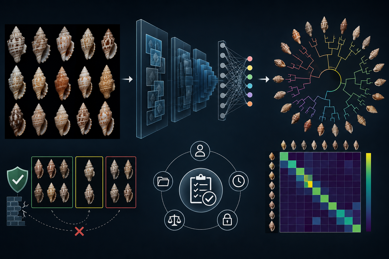
Supplementary Figure SM1.
Relationship between automated thresholds and final quality-control decisions.
Some conditions caused explicit processing failure; others generated diagnostic
warnings. Warning status alone neither accepted nor rejected an image.
Analytical entry ultimately required reviewer-accepted, analysis-ready RGB,
shape and pattern components.
Processing provenance and versioning
Each committed processing stage stored a run identifier, algorithm version,
eligibility rule and serialized parameter set. Detection runs additionally stored
the segmentation-model path and SHA-256 digest. Individual transformed images
retained parent-image identifiers, transformation type, generation method and
version, dimensions, file hash, processing status, QC status and analytical
readiness. Orientation transformations recorded their geometric matrix, and shape
and pattern derivatives retained the accepted orientation as their parent.
Reprocessing did not overwrite previously generated derivatives. Orientation
corrections and deliberate reruns created new versioned transformed images;
superseded derivatives were retained but marked non-analysis-ready. This
provenance structure allowed the final analytical cohort to be restricted to
complete accepted image lineages while preserving earlier processing and review
decisions for audit.
SM3. Operational catalogue of physical and biological traits
Supplementary Table S1 lists all 41 predefined trait fields. Measurements
were made only within the accepted shell mask or from specimen metadata.
Shape traits used the binary silhouette, pattern traits used the
luminance-normalized pattern representation and colour traits used the
masked RGB representation. Unless otherwise indicated, proportional
measurements are dimensionless and range from 0 to 1.
The catalogue contains 41 measured fields and three fields requiring future
annotation. “Primary” denotes a measurement used to describe biological
phenotype. “Exploratory” denotes a reproducible image descriptor whose
biological interpretation has not been independently validated. “Legacy”
denotes a field retained for comparison but excluded from independent
evidence counts.
Supplementary Table S1. Operational definitions
of the 41 physical and image-derived phenotype traits.
Trait
Operational definition
Input
Unit
Status and qualification
A. Conventional morphometrics — four measured traits
Stored shell length
Maximum physical shell length recorded in the specimen
metadata. It was never inferred from the standardized canvas.
Specimen metadata
mm
Primary; missing values were not imputed
Shell width
Width propagated through the accepted image lineage from
recorded shell length and the segmented shell’s short- to
long-axis geometry.
Metadata and silhouette geometry
mm
Primary but derived and view-dependent; not an independent
calliper measurement
Physical aspect ratio
Stored shell length divided by derived shell width.
Conventional morphometrics
Ratio
Measured; strongly overlaps shell slenderness and was not
counted as independent support
Cross-intersection ratio
Position of the maximum perpendicular short-axis intersection
along the apex-to-base long axis, divided by long-axis length.
Orientation geometry
Proportion
Primary; projection- and view-dependent
B. Initially defined biological traits — five measured traits
Shell slenderness
Apex-to-base long-axis length divided by maximum perpendicular
short-axis length.
Orientation geometry
Ratio
Primary; geometrically redundant with physical aspect ratio
Shoulder width ratio
Shell-mask width at 25% of shell height divided by mask width
at 50% of shell height.
Binary silhouette
Ratio
Primary; view-dependent
Pattern density
Fraction of masked pattern pixels with grayscale intensity
below 100 on the 0–255 scale.
Pattern representation
Proportion
Primary; threshold-dependent
White-pattern coverage
Fraction of masked pattern pixels with grayscale intensity
above 200 on the 0–255 scale.
Pattern representation
Proportion
Primary; threshold-dependent
Mean surface hue
Mean HSV hue angle of pixels inside the segmented shell.
Repeated-image values were combined using a circular mean.
Masked RGB representation
Degrees
Primary circular variable
C. Expanded shape geometry — eight measured traits
Relative spire height
Distance from the apex to the detected upper-body shoulder,
divided by shell-mask height. The shoulder was identified as
the maximum smoothed width within the upper 4–45% of shell
height.
Binary silhouette
Proportion
Primary; view- and shoulder-detection-dependent
Spire included angle
Included angle formed by the apex and the left and right shell
outline at the detected shoulder row.
Binary silhouette
Degrees
Primary; dependent on detected shoulder position
Maximum-width position
Vertical position of the overall maximum smoothed mask width
divided by shell-mask height.
Binary silhouette
Proportion
Primary; view-dependent
Shoulder angularity
Absolute change in the local mask-width slope immediately
above and below the detected shoulder, normalized by shell
height and maximum width.
Binary silhouette
Index
Primary; detector-dependent
Outline solidity
Area of the largest shell-mask component divided by the area
of its convex hull.
Binary silhouette
Proportion
Primary
Outline compactness
Four times π multiplied by shell-mask area and divided by
squared outline perimeter.
Binary silhouette
Index
Primary; affected by small-scale mask irregularity
Outline asymmetry
Mean absolute displacement of row-wise shell centres from the
median long-axis centre, divided by maximum shell width.
Binary silhouette
Proportion
Primary; sensitive to oblique projection
Body taper ratio
Smoothed shell-mask width at 75% of shell height divided by
width at 35% of shell height.
Binary silhouette
Ratio
Primary; view-dependent
D. Pattern organization — nine measured traits
Continuous band strength
Standard deviation of the detrended horizontal mean-luminance
profile divided by 255. The trend was estimated by Gaussian
smoothing across shell height.
Pattern representation
Index
Primary continuous replacement for binary band presence
Detected band count
Number of prominent dark minima in the detrended horizontal
luminance profile. Minima were separated by at least 6% of
shell height and required prominence of at least four
grayscale units or 0.8 residual standard deviations,
whichever was larger.
Pattern representation
Count
Primary but threshold-dependent
Upper-third pattern density
Fraction of shell pixels darker than 100 within the upper
third of shell height.
Pattern representation
Proportion
Primary
Middle-third pattern density
Fraction of shell pixels darker than 100 within the middle
third of shell height.
Pattern representation
Proportion
Primary
Lower-third pattern density
Fraction of shell pixels darker than 100 within the lower
third of shell height.
Pattern representation
Proportion
Primary
Reticulation edge density
Fraction of shell-mask pixels identified as edges using a
Canny detector with thresholds 60 and 140.
Pattern representation
Proportion
Primary image descriptor; includes all detectable internal
pattern edges
Dark-fragment density
Number of valid connected dark components per 10,000
shell-mask pixels. Dark components used the same intensity
threshold as pattern density.
Pattern representation
Count per 10,000 pixels
Primary but threshold-dependent
Median dark-fragment size
Median area of valid dark connected components divided by
total shell-mask area. Components smaller than four pixels or
approximately 0.015% of shell area and components larger than
8% of shell area were excluded.
Pattern representation
Relative area
Primary but component-filter-dependent
Pattern luminance entropy
Shannon entropy of the 256-level grayscale histogram within
the shell mask.
Pattern representation
Bits
Primary; describes tonal diversity rather than spatial
arrangement alone
E. Tent-like element geometry — four measured traits
Tent-like element count
Number of enclosed pale components with grayscale intensity
above 170, HSV saturation below 150 on the 0–255 scale,
relative area within the accepted component range, solidity
of at least 0.68 and polygonal complexity of 3–12 vertices.
Pattern representation
Count
Exploratory automated detector
Tent-like element density
Number of detected tent-like elements per 10,000 shell-mask
pixels.
Pattern representation
Count per 10,000 pixels
Exploratory automated detector
Mean relative tent size
Mean area of detected tent-like elements divided by total
shell-mask area; recorded as zero when no element was detected.
Pattern representation
Relative area
Exploratory automated detector
Median relative tent size
Median area of detected tent-like elements divided by total
shell-mask area; recorded as zero when no element was detected.
Pattern representation
Relative area
Exploratory automated detector
F. Expanded colour phenotype — nine measured traits
Mean saturation
Arithmetic mean of HSV saturation values inside the shell
mask, scaled to 0–1.
Masked RGB representation
Proportion
Primary image-derived colour descriptor
Mean surface lightness
Mean CIELAB lightness inside the shell mask, scaled to 0–1.
Masked RGB representation
Proportion
Sensitive to residual illumination differences
Hue dispersion
One minus the circular resultant length of hue angles among
shell pixels with HSV saturation greater than 0.08.
Masked RGB representation
Circular variance
Primary circular colour-diversity measure
Mean chroma
Mean radial distance from the neutral point in the CIELAB
a–b plane.
Masked RGB representation
CIELAB chroma
Primary image-derived colour descriptor
Surface colour contrast
Standard deviation of CIELAB lightness inside the shell mask,
scaled to 0–1.
Masked RGB representation
Proportion
Primary tonal-contrast descriptor
Colour heterogeneity
Root-mean-square CIELAB distance of shell pixels from the
masked-shell mean colour.
Masked RGB representation
CIELAB distance
Primary multivariate colour-diversity descriptor
Brown coverage
Fraction of shell pixels with hue between 5° and 65°,
saturation above 0.18 and brightness below 0.68.
Masked RGB representation
Proportion
Exploratory rule-based colour category
Orange coverage
Fraction of shell pixels with hue between 5° and 65°,
saturation above 0.18 and brightness of at least 0.68.
Masked RGB representation
Proportion
Exploratory rule-based colour category
Violet coverage
Fraction of shell pixels with hue between 250° and 330° and
saturation above 0.12.
Masked RGB representation
Proportion
Exploratory rule-based colour category
G. Legacy fields — two measured fields
Legacy spire-height field
Historical field containing a copy of the cross-intersection
ratio rather than an independent estimate of spire height.
Orientation geometry
Proportion
Legacy and redundant; excluded from independent evidence
counts
Legacy binary band presence
Historical binary indicator based on whether mean absolute
differences in the horizontal luminance profile exceeded the
original threshold.
Pattern representation
Binary
Legacy and superseded by continuous band strength and band
count
Measurement pooling and validity
Measurements were calculated independently for each accepted image.
When several accepted images represented the same physical specimen in
the same anatomical view, valid values were averaged. Mean hue was the
exception and was combined by circular mean. Dorsal and apertural values
were not averaged together. If an input image or shell mask was unreadable,
dimensionally inconsistent or empty, measurements requiring that input were
marked invalid. Missing physical measurements and invalid image-derived
values were not imputed.
Interpretive limitations
Several traits share pixels, thresholds or mathematical components and are
therefore correlated by construction. The number of individually supported
traits was not interpreted as the number of independent biological
differences. Evidence summaries emphasized non-redundant phenotype modules,
effect sizes and consistency across shape, pattern and colour. Tent-like
elements and rule-based colour coverages were treated as exploratory until
independently validated against manual annotations.
SM4. Embedding and dimensionality-reduction implementation details
This section records the computational identifiers, artifact contracts and
projection parameters associated with the embedding and dimensionality-reduction
workflow. The statistical role of the embeddings, feature standardization,
principal-component retention rule and restriction of nonlinear projections to
exploratory visualization are described in the main Methods and are not repeated
here.
SM4.1 Registered embedding-extraction contract
Embedding extraction was implemented by
extract_pennaceus_dinov3.py, extractor version
2.0.1. The registered model key was
dinov3_vits16_cls336_v2, using the DINOv3 preset
dinov3_vit_small_lvd1689m
[4]. The preprocessing-contract identifier was
keras_hub_dinov3_converter_explicit336_v2.
The extraction implementation defined the following immutable model contract:
TensorFlow/KerasHub framework, 336 × 336-pixel input,
class-token pooling, 384 output dimensions, float32 raw vectors
and a separately stored L2-normalized float32 representation.
The model-weight digest encoded in the supplied extraction contract was:
Each committed extraction run produced an immutable artifact directory
containing manifest.csv, cohort_manifest.csv,
embeddings.raw.float32.npy,
embeddings.l2.float32.npy,
transformed_image_ids.uint64.npy,
items.csv, metadata.json,
result.json, run.log and
SHA256SUMS. Individual embedding-vector records additionally
stored SHA-256 digests for both their raw and L2-normalized byte
representations.
Extraction metadata recorded the embedding run identifier and run name,
representation-run identifier, host and platform, model contract,
model-contract SHA-256, manifest SHA-256, embedding dimensions and dtype,
together with the installed TensorFlow, Keras, KerasHub, NumPy and Pillow
versions. These values remained attached to the versioned extraction run
rather than being inferred later from the analysis environment.
SM4.2 Frozen input arrays used for dimensionality reduction
The dimensionality-reduction runs used the frozen reviewed specimen–view
cohort:
pennaceus_reviewed_assignments_v1_20260813
The cohort contained 1,862 aligned specimen–view units from 1,000
physical specimens. All three streams used exactly the same ordered
analysis_unit_id vector. The dimensionality-reduction worker read
the following L2-normalized cohort arrays:
Before any dimensionality-reduction calculation, the worker verified the
cohort's complete SHA256SUMS manifest. It then required the
analysis_unit_ids.uint64.npy sequence to agree exactly with the
ordered database analysis units, rejected non-finite feature values, and
required the maximum absolute departure of input-vector L2 norms from unity
to be no greater than 10−4.
The SHA-256 digest of each source array was taken from the verified cohort
checksum manifest, or recalculated directly if not present there, and stored
in Pennaceus_DimRedRun.source_array_sha256 together with the
corresponding source_array_path. The supplied fixed publication
pages preserve the run keys and dimensionality results but do not render the
three 64-character source-array digests themselves.
SM4.3 Dimensionality-reduction run identifiers and retained dimensions
Dimensionality reduction was performed by the versioned worker
compute_dimensionality_reduction_v2.py. The three fixed
publication snapshots identify the following immutable run keys:
Stream
Dimensionality-reduction run key
k80
k85
k90
RGB
reviewed_assignments_dimred_v1_20260813_rgb
41
56
80
Shape
reviewed_assignments_dimred_v1_20260813_shape
15
19
29
Pattern
reviewed_assignments_dimred_v1_20260813_pattern
42
57
81
Table SM4.1.
Dimensionality-reduction runs associated with the reviewed frozen cohort.
Values are the exact numbers of PCs required to reach the three stored
cumulative-variance thresholds. The
k85 column identifies the coordinate count supplied
to the primary downstream inference.
The database contract for these runs recorded
sklearn.StandardScaler(with_mean=True,with_std=True) and
sklearn.PCA(svd_solver=full). PCA component eigenvalues and
explained-variance ratios were written to
Pennaceus_PCAComponent; retained specimen–view PC scores
were written to Pennaceus_PCAScore.
SM4.4 Exact exploratory projection parameters
UMAP and t-SNE were generated from the same standardized
384-dimensional specimen–view matrices used as PCA input. Their
parameter dictionaries were fixed in the dimensionality-reduction worker and
stored with each run.
Projection
Parameter
Value
UMAP
n_components
2
n_neighbors
15
min_dist
0.1
metric
euclidean
random_state
42
n_jobs
1
t-SNE
n_components
2
perplexity
30.0
max_iter
1000
init
pca
learning_rate
auto
random_state
42
Table SM4.2.
Exact parameterization of the exploratory nonlinear projections stored
with each dimensionality-reduction run. The same settings were applied
independently to RGB, shape and pattern.
The stored two-dimensional coordinates, together with PC1–PC3, were
registered in Pennaceus_DimRedCoordinate for every
analysis_unit_id. UMAP was run with a single worker
(n_jobs=1) and both nonlinear methods used
random_state=42.
SM4.5 Software-version provenance
Software provenance was stored at the computational stage that generated the
corresponding artifacts. The embedding extractor recorded versions for
TensorFlow, Keras, KerasHub, NumPy and Pillow, together with the execution host
and platform. The dimensionality-reduction worker independently recorded
NumPy, scikit-learn and umap-learn versions in
Pennaceus_DimRedRun.software_versions_json.
The fixed HTML publication snapshots supplied with the present manuscript do
not render the literal package-version strings from these registry fields.
Consequently, no software version has been reconstructed from installation
dates or from a different execution environment. The exact values remain
attached to the corresponding immutable run records.
SM4.6 Array and database lineage
The dimensionality-reduction worker enforced the following provenance chain
before writing any projection result. The requested analytical cohort had to
have status frozen; its checksum manifest had to validate; the
ordered analysis_unit_ids.uint64.npy array had to match the
included database analysis units exactly; and the selected representation
array had to satisfy its dimensionality, dtype, finiteness and L2-norm
contracts.
On creation of a dimensionality-reduction run, the cohort identifier,
embedding-model identifier, representation stream, sample and feature counts,
scaler and PCA contracts, UMAP and t-SNE parameter JSON, software-version JSON,
source-array path and source-array SHA-256 were written to
Pennaceus_DimRedRun. PCA eigenvalues, retained PC scores and
visualization coordinates were then linked back to the same
dimred_run_id and analysis_unit_id values.
Figure SM4.1.
Computational provenance of the embedding and dimensionality-reduction
workflow. The registered image-embedding contract feeds a checksum-protected
frozen specimen–view cohort. RGB, shape and pattern use aligned source
arrays and separate immutable dimensionality-reduction run keys. Integrity
checks precede PCA and exploratory nonlinear projection, and all resulting
coordinates remain linked to the corresponding run and analytical-unit
identifiers.
Reproducibility boundary.
The stable cohort key and dimensionality-reduction run keys identify the
publication-facing analysis state. The run registry additionally retains
exact source-array hashes and package-version metadata. Values not exposed
by the supplied fixed HTML snapshots were not reconstructed or inferred
from another computing environment.
Supplementary Results
S1. Complete coverage and descriptive distributions of measured shell traits
This section provides the complete descriptive record for the 41 physical and
image-derived phenotype fields used in the study. It supplements the selected
distributions reported in Result 1 and does not introduce an additional
inferential analysis. Operational definitions, units and measurement algorithms
for the individual fields are provided in Supplementary Table S1.
S1.1 Specimen-level construction and coverage
Descriptive statistics were calculated once per physical specimen. When an
apertural specimen–view was available it supplied the specimen-level
measurement; a dorsal observation was used only when no apertural observation
was available. The resulting descriptive dataset therefore comprised 934
apertural-preferred and 66 dorsal-fallback specimen records, for a total of
1,000 physical specimens. Dorsal and apertural measurements were not averaged
together for this summary.
Thirty-eight of the 41 measured fields had complete specimen-level coverage.
Stored shell length, derived shell width and physical aspect ratio were available
for 837 specimens (83.7%); the remaining 163 specimens lacked the stored
physical-length measurement required for those fields. The image-derived
measurements and cross-intersection ratio were available for all 1,000 physical
specimens. Missing values were not imputed.
Supplementary Table S1 reports the median, interquartile range and complete
observed range of each field. The complete range is retained here for audit,
including isolated extreme measurements. In the main Results, selected traits
were instead summarized using their central 98% range when a robust description
of the bulk of the distribution was more informative than the absolute
endpoints. No observation was removed solely because it occupied an extreme
position in one of these descriptive distributions.
Figure S1.
Coverage and analytical status of the measured-trait catalogue.
Thirty-eight fields were available for all 1,000 physical specimens;
shell length and the two fields dependent on it were available for
837 specimens. The complete catalogue includes primary, derived or
duplicated, exploratory and legacy measurements; these categories were
retained in the descriptive supplement rather than filtering the table to
the 29-trait primary phenotype space.
S1.2 Distributional features relevant to interpretation
The complete distributions included both comparatively constrained variables
and strongly asymmetric measurements. Shell outline solidity, compactness and
body taper occupied relatively narrow ranges around their central values,
whereas shoulder angularity, dark-fragment density, tent-like-element
measurements, hue dispersion and several rule-based colour-coverages contained
longer tails. Violet coverage was concentrated close to zero, while the legacy
binary band-presence field was constant at zero.
These distributional properties were treated descriptively. No generic
statistical outlier threshold was applied across the 41 traits, and the
observed endpoints reported in Supplementary Table S1 were not automatically
excluded from later analyses. Analysis-specific complete-case, estimability and
robustness rules are described with the corresponding methods.
Mean surface hue requires separate interpretation because it is circular.
Its median, interquartile range and observed degree range are included in
Supplementary Table S1 only as convenient descriptive summaries. Inferential
analyses requiring hue used the circular treatment specified in the main
Methods rather than treating the degree scale as an unrestricted linear
variable.
S1.3 Complete descriptive trait catalogue
Module
Trait
Analytical status
Valid specimens
Coverage
Median
Interquartile range
Observed range
Conventional morphometrics
Size
Shell length (mm)
Primary
837
83.7%
50.0
46.0–54.8
24.3–77.3
Size
Derived shell width (mm)
Derived
837
83.7%
24.39
22.39–27.11
11.66–42.80
Shape
Physical aspect ratio
Derived / redundant
837
83.7%
2.039
1.892–2.162
1.572–2.650
Shape
Cross-intersection ratio
Primary
1,000
100%
0.280
0.257–0.303
0.006–0.776
Initially defined biological traits
Shape
Shell slenderness
Primary
1,000
100%
2.026
1.885–2.154
1.571–2.650
Shape
Shoulder width ratio
Primary
1,000
100%
1.084
1.062–1.119
0.934–1.228
Pattern
Pattern density
Primary
1,000
100%
0.321
0.242–0.415
0.079–0.809
Pattern
White-pattern coverage
Primary
1,000
100%
0.115
0.066–0.188
0–0.527
Colour
Mean surface hue (degrees)
Primary; circular
1,000
100%
59.1
39.9–105.9
13.9–303.8
Expanded shape geometry
Shape
Relative spire height
Primary
1,000
100%
0.295
0.271–0.316
0.144–0.420
Shape
Spire included angle (degrees)
Primary
1,000
100%
80.0
75.0–87.8
53.2–124.1
Shape
Maximum-width position
Redundant
1,000
100%
0.295
0.271–0.316
0.144–0.420
Shape
Shoulder angularity
Primary
1,000
100%
0.387
0.233–0.542
0.001–2.616
Shape
Outline solidity
Primary
1,000
100%
0.995
0.993–0.997
0.932–1.002
Shape
Outline compactness
Primary
1,000
100%
0.682
0.667–0.696
0.497–0.736
Shape
Outline asymmetry
Primary
1,000
100%
0.0132
0.0116–0.0151
0.0060–0.0453
Shape
Body taper ratio
Primary
1,000
100%
0.694
0.672–0.714
0.551–0.803
Pattern organization
Pattern
Continuous band strength
Primary
1,000
100%
0.0482
0.0432–0.0543
0.0239–0.0975
Pattern
Detected band count
Primary
1,000
100%
8
7–9
1–13
Pattern
Upper-third pattern density
Primary
1,000
100%
0.309
0.219–0.405
0.021–0.871
Pattern
Middle-third pattern density
Primary
1,000
100%
0.368
0.275–0.484
0.055–0.915
Pattern
Lower-third pattern density
Primary
1,000
100%
0.254
0.173–0.379
0.006–0.805
Pattern
Reticulation edge density
Primary
1,000
100%
0.197
0.161–0.228
0.028–0.366
Pattern
Dark-fragment density
Primary
1,000
100%
4.97
2.44–9.58
0.06–47.78
Pattern
Median dark-fragment size
Primary
1,000
100%
0.000308
0.000266–0.000382
0.000154–0.002031
Pattern
Pattern luminance entropy (bits)
Primary
1,000
100%
7.571
7.463–7.652
6.707–7.762
Exploratory tent-like element measurements
Tent-like elements
Element count
Exploratory
1,000
100%
64.5
36–91
0–298
Tent-like elements
Element density
Exploratory
1,000
100%
7.98
4.38–13.41
0–94.69
Tent-like elements
Median relative element size
Exploratory
1,000
100%
0.000642
0.000457–0.000943
0–0.069412
Tent-like elements
Mean relative element size
Exploratory
1,000
100%
0.001702
0.001086–0.002534
0–0.069412
Expanded colour phenotype
Colour
Mean saturation
Primary
1,000
100%
0.317
0.254–0.404
0.102–0.752
Colour
Mean lightness
Primary
1,000
100%
0.548
0.454–0.621
0.192–0.840
Colour
Hue dispersion
Primary
1,000
100%
0.049
0.019–0.152
0.002–0.951
Colour
Mean chroma
Primary
1,000
100%
15.45
11.55–21.28
4.26–53.79
Colour
Surface colour contrast
Primary
1,000
100%
0.207
0.176–0.235
0.084–0.351
Colour
Colour heterogeneity
Primary
1,000
100%
24.69
22.08–27.09
10.39–37.33
Colour
Brown coverage
Exploratory
1,000
100%
0.340
0.233–0.451
0–0.932
Colour
Orange coverage
Exploratory
1,000
100%
0.085
0.021–0.213
0–0.930
Colour
Violet coverage
Exploratory
1,000
100%
0.00028
0–0.00500
0–0.651
Legacy fields
Legacy
Legacy spire-height field
Legacy / redundant
1,000
100%
0.280
0.257–0.303
0.006–0.776
Legacy
Legacy binary band presence
Legacy / superseded
1,000
100%
0
0–0
0–0
Supplementary Table S1.
Coverage and descriptive distributions of all 41 measured phenotype
fields. Statistics use one record per physical specimen, preferentially
the apertural specimen–view and otherwise the dorsal specimen–view.
Proportions and relative areas are shown on their original 0–1
scale. Mean surface hue is circular; the displayed linear quantiles are
descriptive only. Analytical status indicates whether a field belonged
to the primary phenotype catalogue or was retained as a derived,
duplicated, exploratory or legacy measurement.
Descriptive-data qualifications
Values of outline solidity slightly above 1.0 arose from raster contour
and convex-hull discretization and were treated as numerical approximation
around the theoretical upper limit rather than as biologically meaningful
solidity values greater than one.
Physical aspect ratio closely reproduces shell slenderness, maximum-width
position is identical to relative spire height in the present measurements,
the legacy spire-height field reproduces the cross-intersection ratio, and
the legacy binary band field is constant. Their presence in Supplementary
Table S2 preserves the complete measured-data record but does not give
these fields independent evidential weight.
The tent-like-element measurements and rule-based brown, orange and violet
coverages remain exploratory image descriptors. Their complete
distributions are reported for transparency, but their inclusion in this
descriptive table does not convert them into independently validated
morphological characters.
Supplementary scope.
This section documents coverage and observed trait distributions only.
Trait covariance and redundancy, trait–embedding associations,
phenotype-label comparisons and anatomical-view effects are evaluated in
their dedicated analyses and are not repeated here.
S2. Complete trait–embedding associations
The relationship between directly measured shell phenotype and the image-derived embedding spaces
was evaluated for the RGB, silhouette-shape and luminance-normalized pattern representations.
The principal Results report only selected biologically informative associations. This supplementary
section provides a complete trait-level summary across all three representations without introducing
an additional statistical analysis or an additional criterion for selecting biologically important
relationships.
Forty of the 41 measured fields were statistically estimable. The legacy binary band-presence
field was constant and therefore had no estimable association. For each of the remaining traits,
Supplementary Table S2.1 reports the retained principal component having the largest absolute
partial Pearson correlation within each representation. The retained embedding spaces contained
56 RGB PCs, 19 shape PCs and 57 pattern PCs. The complete calculation therefore comprised
5,280 stored trait–PC association records
(40 × [56 + 19 + 57]).
Interpretation of the table.
The signed partial r describes the association between a measured trait and the selected
embedding PC after adjustment for geographic region, repository provider and anatomical view.
“PC variance” is the proportion of total variance in that representation's embedding
space represented by the selected PC. These quantities describe different statistical objects.
Shared residual variance for a particular trait–PC pair is
r2; exact full-precision coefficients and their squared values are retained in
the complete machine-readable association records rather than being recalculated from the
three-decimal display values below.
FDR q-values retain the correction scheme defined in the main Methods: correction was
performed across all retained PCs within one trait and one representation. The values therefore
do not represent a false-discovery-rate correction across the complete trait-by-PC matrix.
Sample size refers to specimen–view units with a valid value for the corresponding trait.
Physical-size measurements were available for 1,603 units; the other estimable traits represented
1,862 units.
Measured trait
n
RGB
Shape
Pattern
Initially defined biological traits
Shell slenderness slenderness_ratio
1,862
PC3
partial r = −0.670
PC variance = 6.61% q < 0.001
PC2
partial r = −0.633
PC variance = 14.08% q < 0.001
PC3
partial r = −0.668
PC variance = 6.55% q < 0.001
Shoulder width ratio shoulder_width_ratio
1,862
PC3
partial r = +0.480
PC variance = 6.61% q < 0.001
PC2
partial r = +0.548
PC variance = 14.08% q < 0.001
PC3
partial r = +0.480
PC variance = 6.55% q < 0.001
Pattern density pattern_density
1,862
PC1
partial r = +0.517
PC variance = 15.15% q < 0.001
PC2
partial r = −0.230
PC variance = 14.08% q < 0.001
PC1
partial r = +0.530
PC variance = 15.25% q < 0.001
White coverage white_pattern_coverage
1,862
PC1
partial r = −0.483
PC variance = 15.15% q < 0.001
PC6
partial r = +0.148
PC variance = 4.81% q < 0.001
PC1
partial r = −0.487
PC variance = 15.25% q < 0.001
Mean surface hue mean_hue
1,862
PC4
partial r = +0.267
PC variance = 4.81% q < 0.001
PC15
partial r = +0.096
PC variance = 1.31% q < 0.001
PC4
partial r = +0.237
PC variance = 4.67% q < 0.001
Conventional morphometrics
Stored shell length shell_length_mm
1,603
PC4
partial r = +0.238
PC variance = 4.81% q < 0.001
PC6
partial r = +0.289
PC variance = 4.81% q < 0.001
PC4
partial r = +0.233
PC variance = 4.67% q < 0.001
Stored shell width shell_width_mm
1,603
PC8
partial r = −0.237
PC variance = 2.36% q < 0.001
PC5
partial r = −0.292
PC variance = 5.06% q < 0.001
PC3
partial r = +0.211
PC variance = 6.55% q < 0.001
Physical aspect ratio physical_aspect_ratio
1,603
PC3
partial r = −0.709
PC variance = 6.61% q < 0.001
PC2
partial r = −0.622
PC variance = 14.08% q < 0.001
PC3
partial r = −0.707
PC variance = 6.55% q < 0.001
Cross Intersection Ratio cross_position_ratio
1,862
PC42
partial r = +0.140
PC variance = 0.41% q < 0.001
PC2
partial r = −0.221
PC variance = 14.08% q < 0.001
PC3
partial r = −0.131
PC variance = 6.55% q < 0.001
Shape geometry
Relative spire height relative_spire_height
1,862
PC3
partial r = −0.363
PC variance = 6.61% q < 0.001
PC2
partial r = −0.518
PC variance = 14.08% q < 0.001
PC3
partial r = −0.365
PC variance = 6.55% q < 0.001
Spire included angle spire_angle_deg
1,862
PC3
partial r = +0.585
PC variance = 6.61% q < 0.001
PC2
partial r = +0.685
PC variance = 14.08% q < 0.001
PC3
partial r = +0.585
PC variance = 6.55% q < 0.001
Maximum-width position max_width_position_ratio
1,862
PC3
partial r = −0.362
PC variance = 6.61% q < 0.001
PC2
partial r = −0.517
PC variance = 14.08% q < 0.001
PC3
partial r = −0.364
PC variance = 6.55% q < 0.001
Shoulder angularity shoulder_angularity
1,862
PC12
partial r = +0.119
PC variance = 1.65% q < 0.001
PC6
partial r = −0.142
PC variance = 4.81% q < 0.001
PC4
partial r = −0.107
PC variance = 4.67% q < 0.001
Outline solidity outline_solidity
1,862
PC3
partial r = −0.208
PC variance = 6.61% q < 0.001
PC2
partial r = −0.299
PC variance = 14.08% q < 0.001
PC3
partial r = −0.206
PC variance = 6.55% q < 0.001
Outline compactness outline_compactness
1,862
PC3
partial r = +0.305
PC variance = 6.61% q < 0.001
PC5
partial r = −0.430
PC variance = 5.06% q < 0.001
PC3
partial r = +0.306
PC variance = 6.55% q < 0.001
Outline asymmetry outline_asymmetry
1,862
PC3
partial r = +0.311
PC variance = 6.61% q < 0.001
PC1
partial r = +0.568
PC variance = 20.42% q < 0.001
PC3
partial r = +0.316
PC variance = 6.55% q < 0.001
Body taper ratio body_taper_ratio
1,862
PC4
partial r = +0.285
PC variance = 4.81% q < 0.001
PC6
partial r = +0.629
PC variance = 4.81% q < 0.001
PC4
partial r = +0.293
PC variance = 4.67% q < 0.001
Pattern organization
Continuous band strength band_strength
1,862
PC6
partial r = +0.271
PC variance = 3.29% q < 0.001
PC11
partial r = +0.107
PC variance = 2.41% q < 0.001
PC8
partial r = −0.212
PC variance = 2.33% q < 0.001
Detected band count band_count
1,862
PC1
partial r = −0.458
PC variance = 15.15% q < 0.001
PC1
partial r = −0.190
PC variance = 20.42% q < 0.001
PC1
partial r = −0.449
PC variance = 15.25% q < 0.001
Upper-third pattern density upper_pattern_density
1,862
PC3
partial r = −0.473
PC variance = 6.61% q < 0.001
PC2
partial r = −0.233
PC variance = 14.08% q < 0.001
PC3
partial r = −0.451
PC variance = 6.55% q < 0.001
Middle-third pattern density middle_pattern_density
1,862
PC1
partial r = +0.487
PC variance = 15.15% q < 0.001
PC2
partial r = −0.205
PC variance = 14.08% q < 0.001
PC1
partial r = +0.498
PC variance = 15.25% q < 0.001
Lower-third pattern density lower_pattern_density
1,862
PC1
partial r = +0.553
PC variance = 15.15% q < 0.001
PC2
partial r = −0.164
PC variance = 14.08% q < 0.001
PC1
partial r = +0.562
PC variance = 15.25% q < 0.001
Reticulation edge density reticulation_edge_density
1,862
PC3
partial r = −0.695
PC variance = 6.61% q < 0.001
PC2
partial r = −0.424
PC variance = 14.08% q < 0.001
PC3
partial r = −0.696
PC variance = 6.55% q < 0.001
Dark-fragment density pattern_fragment_density
1,862
PC6
partial r = −0.375
PC variance = 3.29% q < 0.001
PC14
partial r = +0.106
PC variance = 1.52% q < 0.001
PC7
partial r = −0.340
PC variance = 2.71% q < 0.001
Median dark-fragment size median_dark_fragment_area
1,862
PC3
partial r = +0.274
PC variance = 6.61% q < 0.001
PC2
partial r = +0.112
PC variance = 14.08% q < 0.001
PC3
partial r = +0.269
PC variance = 6.55% q < 0.001
Pattern luminance entropy pattern_entropy
1,862
PC1
partial r = −0.461
PC variance = 15.15% q < 0.001
PC1
partial r = −0.183
PC variance = 20.42% q < 0.001
PC1
partial r = −0.450
PC variance = 15.25% q < 0.001
Tent-like element geometry — exploratory descriptors
Tent-like element count tent_count
1,862
PC3
partial r = −0.455
PC variance = 6.61% q < 0.001
PC1
partial r = −0.258
PC variance = 20.42% q < 0.001
PC3
partial r = −0.468
PC variance = 6.55% q < 0.001
Tent-like element density tent_density
1,862
PC5
partial r = +0.410
PC variance = 4.34% q < 0.001
PC2
partial r = −0.210
PC variance = 14.08% q < 0.001
PC3
partial r = −0.414
PC variance = 6.55% q < 0.001
Median relative tent size median_tent_relative_area
1,862
PC3
partial r = +0.161
PC variance = 6.61% q < 0.001
PC1
partial r = +0.119
PC variance = 20.42% q < 0.001
PC3
partial r = +0.161
PC variance = 6.55% q < 0.001
Mean relative tent size mean_tent_relative_area
1,862
PC3
partial r = +0.319
PC variance = 6.61% q < 0.001
PC1
partial r = +0.179
PC variance = 20.42% q < 0.001
PC3
partial r = +0.320
PC variance = 6.55% q < 0.001
Expanded colour phenotype
Mean saturation mean_saturation
1,862
PC1
partial r = +0.610
PC variance = 15.15% q < 0.001
PC6
partial r = −0.155
PC variance = 4.81% q < 0.001
PC1
partial r = +0.603
PC variance = 15.25% q < 0.001
Mean surface lightness mean_lightness
1,862
PC1
partial r = −0.454
PC variance = 15.15% q < 0.001
PC2
partial r = +0.171
PC variance = 14.08% q < 0.001
PC1
partial r = −0.467
PC variance = 15.25% q < 0.001
Hue dispersion hue_dispersion
1,862
PC4
partial r = +0.293
PC variance = 4.81% q < 0.001
PC4
partial r = −0.115
PC variance = 7.27% q < 0.001
PC4
partial r = +0.264
PC variance = 4.67% q < 0.001
Mean chroma mean_chroma
1,862
PC1
partial r = +0.473
PC variance = 15.15% q < 0.001
PC15
partial r = −0.158
PC variance = 1.31% q < 0.001
PC1
partial r = +0.459
PC variance = 15.25% q < 0.001
Surface colour contrast colour_contrast
1,862
PC6
partial r = +0.461
PC variance = 3.29% q < 0.001
PC4
partial r = −0.132
PC variance = 7.27% q < 0.001
PC1
partial r = −0.372
PC variance = 15.25% q < 0.001
Colour heterogeneity colour_heterogeneity
1,862
PC6
partial r = +0.380
PC variance = 3.29% q < 0.001
PC1
partial r = −0.159
PC variance = 20.42% q < 0.001
PC1
partial r = −0.332
PC variance = 15.25% q < 0.001
Brown coverage brown_coverage exploratory
1,862
PC1
partial r = +0.440
PC variance = 15.15% q < 0.001
PC2
partial r = −0.173
PC variance = 14.08% q < 0.001
PC1
partial r = +0.442
PC variance = 15.25% q < 0.001
Orange coverage orange_coverage exploratory
1,862
PC4
partial r = −0.423
PC variance = 4.81% q < 0.001
PC1
partial r = +0.252
PC variance = 20.42% q < 0.001
PC4
partial r = −0.390
PC variance = 4.67% q < 0.001
Violet coverage violet_coverage exploratory
1,862
PC9
partial r = +0.160
PC variance = 2.18% q < 0.001
PC5
partial r = −0.075
PC variance = 5.06% q = 0.027
PC9
partial r = +0.200
PC variance = 2.21% q < 0.001
Legacy fields
Legacy spire-height field legacy_spire_height_ratio legacy / redundant
1,862
PC42
partial r = +0.140
PC variance = 0.41% q < 0.001
PC2
partial r = −0.221
PC variance = 14.08% q < 0.001
PC3
partial r = −0.131
PC variance = 6.55% q < 0.001
Legacy binary band presence legacy_band_presence legacy / constant
1,862
Not estimable
Not estimable
Not estimable
Supplementary Table S2.1.
Strongest retained embedding-PC association for every measured phenotype field in each of the
RGB, silhouette-shape and luminance-normalized pattern representations. The selected PC is the
component having the largest absolute partial Pearson correlation with the corresponding trait.
Partial correlations are shown with their fitted sign; PCA signs are arbitrary, so sign describes
direction only within the stored orientation of that PC. PC variance is the explained-variance
ratio of the selected embedding PC and is not the variance in that PC explained by the measured
trait. The legacy binary band-presence field was constant and therefore non-estimable.
Complete association records
Supplementary Table S2.1 is a trait-level index of the complete analysis rather than a replacement
for the underlying coefficient matrix. The machine-readable supplementary data retain every
estimable trait–PC combination for all three representations, including representation,
trait identifier, PC index, sample size, PC explained-variance ratio, raw correlation, partial
correlation, analytic probability and within-trait, within-representation FDR-adjusted
q-value. This preserves associations involving lower-variance PCs that are not visible
when only the strongest PC for each trait is printed.
Statistical scope.
This section reports the existing trait–embedding analysis and adds no new hypothesis test,
significance threshold or evidence score. Mean surface hue retains the treatment specified in the
main Methods: valid specimen–view hue values were expressed as shortest signed angular
displacements around their circular centre before entering the linear residualization and
partial-correlation calculation. Analytic significance calculations use specimen–view rows;
residual pairing of dorsal and apertural observations from the same physical specimen is not
explicitly modelled.
Interpretive boundary.
The table documents which individual measured traits correspond most strongly to individual
axes of each embedding representation. It does not estimate how much of the complete embedding
space can jointly be reconstructed from the measured-trait catalogue, and a strong association
does not imply that an embedding PC represents a single biological character. RGB and pattern
are derived from the same shell photographs and their agreement should not be counted as
independent biological evidence.
S3. Complete trait-covariance matrix
The complete covariance structure of the 41 measured phenotype fields was
examined at physical-specimen level to document relationships that are
necessarily summarized only selectively in the main Results. This
supplementary analysis reports the pairwise Spearman correlation structure
underlying the redundancy assessment and the subsequent definition of the
primary measured-trait space. It does not introduce an additional hypothesis
test, correlation threshold or trait-selection rule.
S3.1 Construction of the pairwise correlation matrix
The correlation matrix used the same specimen-level phenotype records as the
measured-trait structure analysis. Repeated photographs had already been
pooled within physical specimen and anatomical view. For this analysis, the
apertural specimen–view was selected when available and the dorsal
specimen–view was used as fallback. Stored shell length was treated as
specimen metadata and was averaged across retained views where required.
Missing measurements were not imputed.
Spearman rank correlations were calculated independently for every pair of
measured fields using all physical specimens having finite values for both
members of that pair. Average ranks were assigned to tied observations.
Consequently, the matrix was pairwise complete rather than restricted to the
837-specimen complete-case population used for the primary trait PCA.
Correlations involving the physical-size fields could contain 837 specimens,
whereas pairs among fields with complete coverage generally contained all
1,000 physical specimens.
The legacy binary band-presence field was constant in the frozen trait run.
Pairwise correlation with a constant variable is not estimable and is
therefore represented as unavailable rather than as a correlation of zero.
The diagonal otherwise represents the usual self-correlation of a variable.
Matrix interpretation
The coefficients describe pairwise monotonic covariance among measured
fields. No value of |ρ| was prespecified as a universal boundary
between redundant and non-redundant traits. Mathematical definition,
measurement provenance and validation status were considered together
with the observed correlations when identifying duplicate fields.
S3.2 Complete correlation matrix
Supplementary Table S3 contains the complete pairwise Spearman correlation
matrix for the 41 measured fields. Cell values are Spearman
ρ. Pairwise sample size is determined by the valid observations
available for the two corresponding traits and therefore is not necessarily
identical throughout the matrix.
Trait
T01
T02
T03
T04
T05
T06
T07
T08
T09
T10
T11
T12
T13
T14
T15
T16
T17
T18
T19
T20
T21
T22
T23
T24
T25
T26
T27
T28
T29
T30
T31
T32
T33
T34
T35
T36
T37
T38
T39
T40
T41
T01 Median dark-fragment size
1.000
0.283
0.280
-0.029
0.045
0.112
-0.150
-0.156
-0.034
0.036
-0.092
0.095
0.176
-0.142
-0.142
-0.091
-0.091
-0.012
-0.037
0.062
-0.011
-0.100
-0.097
-0.146
-0.074
0.017
0.033
-0.096
-0.075
-0.110
-0.090
-0.136
-0.279
-0.155
-0.082
-0.082
-0.043
-0.003
0.065
-0.048
—
T02 Mean relative tent size
0.283
1.000
0.732
0.050
0.237
0.241
-0.342
-0.379
-0.140
0.029
-0.043
0.188
0.299
-0.178
-0.178
-0.169
-0.169
-0.120
-0.019
0.054
-0.037
-0.114
-0.173
-0.220
-0.222
0.160
0.186
-0.255
-0.242
-0.187
-0.012
-0.163
-0.482
-0.270
-0.038
-0.102
0.030
0.008
-0.037
-0.060
—
T03 Median relative tent size
0.280
0.732
1.000
0.158
0.291
0.255
-0.289
-0.310
-0.130
0.006
0.044
0.120
0.239
-0.120
-0.120
-0.097
-0.097
-0.105
-0.077
0.103
-0.017
-0.224
-0.286
-0.231
-0.298
0.277
0.222
-0.255
-0.233
-0.139
-0.014
-0.026
-0.392
-0.019
0.163
0.049
0.096
0.127
-0.051
-0.114
—
T04 Stored shell length
-0.029
0.050
0.158
1.000
0.817
0.091
0.032
0.033
-0.085
0.025
0.348
-0.049
0.006
-0.048
-0.048
-0.039
-0.039
0.129
-0.276
0.296
0.211
-0.352
-0.286
-0.168
0.025
0.079
-0.037
0.042
0.031
0.073
0.019
0.197
0.142
0.186
0.289
0.096
0.104
0.225
-0.037
-0.087
—
T05 Stored shell width
0.045
0.237
0.291
0.817
1.000
0.346
-0.492
-0.492
-0.316
0.175
0.089
0.258
0.409
-0.243
-0.243
-0.176
-0.176
-0.018
-0.236
0.297
0.258
-0.365
-0.300
-0.243
-0.034
0.033
-0.028
-0.043
-0.043
-0.023
0.001
0.002
-0.152
-0.073
0.138
-0.125
-0.038
0.105
-0.126
-0.018
—
T06 Outline compactness
0.112
0.241
0.255
0.091
0.346
1.000
-0.542
-0.520
0.181
-0.215
0.224
-0.045
0.323
-0.045
-0.045
-0.088
-0.088
0.011
-0.070
0.107
-0.005
-0.132
-0.164
-0.178
-0.163
0.094
0.126
-0.190
-0.175
-0.159
-0.041
-0.132
-0.290
-0.144
-0.063
-0.096
-0.005
-0.026
-0.102
0.050
—
T07 Shell slenderness
-0.150
-0.342
-0.289
0.032
-0.492
-0.542
1.000
1.000
0.434
-0.264
0.410
-0.551
-0.764
0.358
0.358
0.237
0.237
0.211
0.057
-0.072
-0.148
0.133
0.074
0.126
0.025
0.135
0.075
0.074
0.061
0.110
0.039
0.287
0.457
0.434
0.176
0.368
0.220
0.134
0.165
-0.049
—
T08 Physical aspect ratio
-0.156
-0.379
-0.310
0.033
-0.492
-0.520
1.000
1.000
0.468
-0.306
0.426
-0.604
-0.786
0.412
0.412
0.283
0.283
0.280
0.017
-0.061
-0.128
0.115
0.055
0.151
0.045
0.115
0.052
0.084
0.069
0.114
0.046
0.311
0.510
0.456
0.204
0.415
0.235
0.150
0.158
-0.058
—
T09 Outline solidity
-0.034
-0.140
-0.130
-0.085
-0.316
0.181
0.434
0.468
1.000
-0.335
0.308
-0.319
-0.305
0.120
0.120
0.012
0.012
0.103
0.136
-0.083
-0.249
0.169
0.051
0.018
-0.117
0.155
0.211
-0.114
-0.103
-0.073
0.059
0.140
0.189
0.209
0.023
0.209
0.108
-0.034
0.030
-0.035
—
T10 Shoulder angularity
0.036
0.029
0.006
0.025
0.175
-0.215
-0.264
-0.306
-0.335
1.000
-0.377
0.327
0.280
-0.215
-0.215
0.084
0.084
-0.161
-0.038
0.020
0.116
-0.064
0.013
0.047
0.116
-0.152
-0.173
0.127
0.121
0.084
0.138
0.048
0.055
-0.138
-0.043
-0.176
-0.168
-0.058
0.016
-0.054
—
T11 Body taper ratio
-0.092
-0.043
0.044
0.348
0.089
0.224
0.410
0.426
0.308
-0.377
1.000
-0.598
-0.383
0.246
0.246
0.103
0.103
0.175
-0.001
0.049
-0.129
-0.041
-0.135
-0.077
-0.126
0.254
0.220
-0.138
-0.141
-0.079
-0.018
0.187
0.124
0.328
0.202
0.292
0.203
0.129
0.006
0.034
—
T12 Shoulder width ratio
0.095
0.188
0.120
-0.049
0.258
-0.045
-0.551
-0.604
-0.319
0.327
-0.598
1.000
0.767
-0.714
-0.714
-0.562
-0.562
-0.269
0.048
-0.021
0.059
-0.005
0.073
-0.078
0.035
-0.118
-0.080
-0.010
0.002
-0.058
0.004
-0.181
-0.279
-0.308
-0.134
-0.274
-0.193
-0.096
-0.146
-0.058
—
T13 Spire included angle
0.176
0.299
0.239
0.006
0.409
0.323
-0.764
-0.786
-0.305
0.280
-0.383
0.767
1.000
-0.855
-0.855
-0.603
-0.603
-0.225
0.017
0.017
0.036
-0.038
0.024
-0.129
-0.042
-0.075
-0.022
-0.098
-0.080
-0.130
0.000
-0.230
-0.390
-0.385
-0.144
-0.303
-0.164
-0.112
-0.152
-0.004
—
T14 Relative spire height
-0.142
-0.178
-0.120
-0.048
-0.243
-0.045
0.358
0.412
0.120
-0.215
0.246
-0.714
-0.855
1.000
1.000
0.729
0.729
0.173
-0.061
0.024
0.056
-0.039
-0.094
0.093
0.028
0.030
-0.003
0.079
0.064
0.101
-0.023
0.121
0.227
0.243
0.083
0.175
0.083
0.054
0.098
0.049
—
T15 Maximum-width position
-0.142
-0.178
-0.120
-0.048
-0.243
-0.045
0.358
0.412
0.120
-0.215
0.246
-0.714
-0.855
1.000
1.000
0.729
0.729
0.173
-0.061
0.024
0.056
-0.039
-0.094
0.093
0.028
0.030
-0.003
0.079
0.064
0.101
-0.023
0.121
0.227
0.243
0.083
0.175
0.083
0.054
0.098
0.049
—
T16 Legacy spire-height field
-0.091
-0.169
-0.097
-0.039
-0.176
-0.088
0.237
0.283
0.012
0.084
0.103
-0.562
-0.603
0.729
0.729
1.000
1.000
0.094
-0.072
0.042
0.144
-0.058
-0.072
0.125
0.092
-0.030
-0.078
0.133
0.105
0.144
0.000
0.126
0.236
0.183
0.105
0.115
0.045
0.057
0.084
0.033
—
T17 Cross Intersection Ratio
-0.091
-0.169
-0.097
-0.039
-0.176
-0.088
0.237
0.283
0.012
0.084
0.103
-0.562
-0.603
0.729
0.729
1.000
1.000
0.094
-0.072
0.042
0.144
-0.058
-0.072
0.125
0.092
-0.030
-0.078
0.133
0.105
0.144
0.000
0.126
0.236
0.183
0.105
0.115
0.045
0.057
0.084
0.033
—
T18 Hue dispersion
-0.012
-0.120
-0.105
0.129
-0.018
0.011
0.211
0.280
0.103
-0.161
0.175
-0.269
-0.225
0.173
0.173
0.094
0.094
1.000
-0.532
0.669
0.478
-0.446
-0.338
-0.275
0.130
-0.006
-0.187
0.184
0.168
0.185
-0.146
0.060
0.107
0.167
0.100
0.179
0.350
0.381
0.162
0.045
—
T19 Orange coverage
-0.037
-0.019
-0.077
-0.276
-0.236
-0.070
0.057
0.017
0.136
-0.038
-0.001
0.048
0.017
-0.061
-0.061
-0.072
-0.072
-0.532
1.000
-0.680
-0.619
0.790
0.447
0.105
-0.355
0.377
0.625
-0.535
-0.484
-0.558
0.332
0.120
0.005
0.051
-0.121
0.052
-0.037
-0.369
-0.127
0.185
—
T20 Mean surface hue
0.062
0.054
0.103
0.296
0.297
0.107
-0.072
-0.061
-0.083
0.020
0.049
-0.021
0.017
0.024
0.024
0.042
0.042
0.669
-0.680
1.000
0.747
-0.636
-0.507
-0.547
0.118
-0.057
-0.253
0.177
0.140
0.210
-0.200
-0.057
-0.071
0.029
0.135
-0.010
0.178
0.347
0.063
-0.119
—
T21 Violet coverage
-0.011
-0.037
-0.017
0.211
0.258
-0.005
-0.148
-0.128
-0.249
0.116
-0.129
0.059
0.036
0.056
0.056
0.144
0.144
0.478
-0.619
0.747
1.000
-0.507
-0.265
-0.215
0.329
-0.296
-0.479
0.385
0.328
0.374
-0.284
-0.144
-0.016
-0.090
0.035
-0.150
0.066
0.252
0.035
-0.133
—
T22 Mean chroma
-0.100
-0.114
-0.224
-0.352
-0.365
-0.132
0.133
0.115
0.169
-0.064
-0.041
-0.005
-0.038
-0.039
-0.039
-0.058
-0.058
-0.446
0.790
-0.636
-0.507
1.000
0.819
0.355
-0.035
0.010
0.241
-0.152
-0.119
-0.232
0.171
-0.011
0.051
-0.106
-0.186
0.014
0.028
-0.382
-0.125
0.207
—
T23 Mean saturation
-0.097
-0.173
-0.286
-0.286
-0.300
-0.164
0.074
0.055
0.051
0.013
-0.135
0.073
0.024
-0.094
-0.094
-0.072
-0.072
-0.338
0.447
-0.507
-0.265
0.819
1.000
0.528
0.340
-0.369
-0.262
0.296
0.301
0.160
-0.015
-0.104
0.068
-0.244
-0.199
-0.048
0.109
-0.164
-0.038
0.142
—
T24 Brown coverage
-0.146
-0.220
-0.231
-0.168
-0.243
-0.178
0.126
0.151
0.018
0.047
-0.077
-0.078
-0.129
0.093
0.093
0.125
0.125
-0.275
0.105
-0.547
-0.215
0.355
0.528
1.000
0.375
-0.409
-0.384
0.459
0.455
0.367
-0.032
0.017
0.217
-0.053
-0.060
0.072
-0.069
-0.115
0.007
-0.031
—
T25 Lower-third pattern density
-0.074
-0.222
-0.298
0.025
-0.034
-0.163
0.025
0.045
-0.117
0.116
-0.126
0.035
-0.042
0.028
0.028
0.092
0.092
0.130
-0.355
0.118
0.329
-0.035
0.340
0.375
1.000
-0.677
-0.745
0.797
0.716
0.460
-0.244
-0.181
0.145
-0.262
-0.112
-0.122
-0.002
0.099
0.057
-0.037
—
T26 White coverage
0.017
0.160
0.277
0.079
0.033
0.094
0.135
0.115
0.155
-0.152
0.254
-0.118
-0.075
0.030
0.030
-0.030
-0.030
-0.006
0.377
-0.057
-0.296
0.010
-0.369
-0.409
-0.677
1.000
0.852
-0.706
-0.681
-0.505
0.273
0.315
0.019
0.448
0.243
0.417
0.380
0.278
0.064
0.057
—
T27 Mean surface lightness
0.033
0.186
0.222
-0.037
-0.028
0.126
0.075
0.052
0.211
-0.173
0.220
-0.080
-0.022
-0.003
-0.003
-0.078
-0.078
-0.187
0.625
-0.253
-0.479
0.241
-0.262
-0.384
-0.745
0.852
1.000
-0.890
-0.844
-0.744
0.308
0.192
-0.096
0.301
0.093
0.180
0.065
-0.151
-0.089
0.128
—
T28 Pattern density
-0.096
-0.255
-0.255
0.042
-0.043
-0.190
0.074
0.084
-0.114
0.127
-0.138
-0.010
-0.098
0.079
0.079
0.133
0.133
0.184
-0.535
0.177
0.385
-0.152
0.296
0.459
0.797
-0.706
-0.890
1.000
0.961
0.847
-0.290
-0.103
0.219
-0.175
-0.014
-0.006
0.068
0.225
0.153
-0.142
—
T29 Middle-third pattern density
-0.075
-0.242
-0.233
0.031
-0.043
-0.175
0.061
0.069
-0.103
0.121
-0.141
0.002
-0.080
0.064
0.064
0.105
0.105
0.168
-0.484
0.140
0.328
-0.119
0.301
0.455
0.716
-0.681
-0.844
0.961
1.000
0.760
-0.279
-0.108
0.184
-0.177
-0.032
-0.003
0.054
0.196
0.163
-0.132
—
T30 Upper-third pattern density
-0.110
-0.187
-0.139
0.073
-0.023
-0.159
0.110
0.114
-0.073
0.084
-0.079
-0.058
-0.130
0.101
0.101
0.144
0.144
0.185
-0.558
0.210
0.374
-0.232
0.160
0.367
0.460
-0.505
-0.744
0.847
0.760
1.000
-0.251
0.007
0.235
-0.039
0.104
0.074
0.122
0.286
0.180
-0.193
—
T31 Dark-fragment density
-0.090
-0.012
-0.014
0.019
0.001
-0.041
0.039
0.046
0.059
0.138
-0.018
0.004
0.000
-0.023
-0.023
0.000
0.000
-0.146
0.332
-0.200
-0.284
0.171
-0.015
-0.032
-0.244
0.273
0.308
-0.290
-0.279
-0.251
1.000
0.714
0.537
0.193
0.019
0.189
-0.016
-0.068
0.036
0.048
—
T32 Tent-like element density
-0.136
-0.163
-0.026
0.197
0.002
-0.132
0.287
0.311
0.140
0.048
0.187
-0.181
-0.230
0.121
0.121
0.126
0.126
0.060
0.120
-0.057
-0.144
-0.011
-0.104
0.017
-0.181
0.315
0.192
-0.103
-0.108
0.007
0.714
1.000
0.736
0.691
0.296
0.481
0.257
0.266
0.195
-0.042
—
T33 Reticulation edge density
-0.279
-0.482
-0.392
0.142
-0.152
-0.290
0.457
0.510
0.189
0.055
0.124
-0.279
-0.390
0.227
0.227
0.236
0.236
0.107
0.005
-0.071
-0.016
0.051
0.068
0.217
0.145
0.019
-0.096
0.219
0.184
0.235
0.537
0.736
1.000
0.502
0.201
0.382
0.159
0.174
0.202
-0.048
—
T34 Tent-like element count
-0.155
-0.270
-0.019
0.186
-0.073
-0.144
0.434
0.456
0.209
-0.138
0.328
-0.308
-0.385
0.243
0.243
0.183
0.183
0.167
0.051
0.029
-0.090
-0.106
-0.244
-0.053
-0.262
0.448
0.301
-0.175
-0.177
-0.039
0.193
0.691
0.502
1.000
0.456
0.567
0.327
0.327
0.141
-0.073
—
T35 Detected band count
-0.082
-0.038
0.163
0.289
0.138
-0.063
0.176
0.204
0.023
-0.043
0.202
-0.134
-0.144
0.083
0.083
0.105
0.105
0.100
-0.121
0.135
0.035
-0.186
-0.199
-0.060
-0.112
0.243
0.093
-0.014
-0.032
0.104
0.019
0.296
0.201
0.456
1.000
0.366
0.256
0.319
-0.200
-0.051
—
T36 Pattern luminance entropy
-0.082
-0.102
0.049
0.096
-0.125
-0.096
0.368
0.415
0.209
-0.176
0.292
-0.274
-0.303
0.175
0.175
0.115
0.115
0.179
0.052
-0.010
-0.150
0.014
-0.048
0.072
-0.122
0.417
0.180
-0.006
-0.003
0.074
0.189
0.481
0.382
0.567
0.366
1.000
0.640
0.617
0.148
0.016
—
T37 Colour heterogeneity
-0.043
0.030
0.096
0.104
-0.038
-0.005
0.220
0.235
0.108
-0.168
0.203
-0.193
-0.164
0.083
0.083
0.045
0.045
0.350
-0.037
0.178
0.066
0.028
0.109
-0.069
-0.002
0.380
0.065
0.068
0.054
0.122
-0.016
0.257
0.159
0.327
0.256
0.640
1.000
0.809
0.222
0.003
—
T38 Surface colour contrast
-0.003
0.008
0.127
0.225
0.105
-0.026
0.134
0.150
-0.034
-0.058
0.129
-0.096
-0.112
0.054
0.054
0.057
0.057
0.381
-0.369
0.347
0.252
-0.382
-0.164
-0.115
0.099
0.278
-0.151
0.225
0.196
0.286
-0.068
0.266
0.174
0.327
0.319
0.617
0.809
1.000
0.280
-0.082
—
T39 Continuous band strength
0.065
-0.037
-0.051
-0.037
-0.126
-0.102
0.165
0.158
0.030
0.016
0.006
-0.146
-0.152
0.098
0.098
0.084
0.084
0.162
-0.127
0.063
0.035
-0.125
-0.038
0.007
0.057
0.064
-0.089
0.153
0.163
0.180
0.036
0.195
0.202
0.141
-0.200
0.148
0.222
0.280
1.000
-0.054
—
T40 Outline asymmetry
-0.048
-0.060
-0.114
-0.087
-0.018
0.050
-0.049
-0.058
-0.035
-0.054
0.034
-0.058
-0.004
0.049
0.049
0.033
0.033
0.045
0.185
-0.119
-0.133
0.207
0.142
-0.031
-0.037
0.057
0.128
-0.142
-0.132
-0.193
0.048
-0.042
-0.048
-0.073
-0.051
0.016
0.003
-0.082
-0.054
1.000
—
T41 Legacy binary band presence
—
—
—
—
—
—
—
—
—
—
—
—
—
—
—
—
—
—
—
—
—
—
—
—
—
—
—
—
—
—
—
—
—
—
—
—
—
—
—
—
—
T01 Median dark-fragment size median_dark_fragment_area
T02 Mean relative tent size mean_tent_relative_area
T03 Median relative tent size median_tent_relative_area
T04 Stored shell length shell_length_mm
T05 Stored shell width shell_width_mm
T06 Outline compactness outline_compactness
T07 Shell slenderness slenderness_ratio
T08 Physical aspect ratio physical_aspect_ratio
T09 Outline solidity outline_solidity
T10 Shoulder angularity shoulder_angularity
T11 Body taper ratio body_taper_ratio
T12 Shoulder width ratio shoulder_width_ratio
T13 Spire included angle spire_angle_deg
T14 Relative spire height relative_spire_height
T15 Maximum-width position max_width_position_ratio
T16 Legacy spire-height field legacy_spire_height_ratio
T17 Cross Intersection Ratio cross_position_ratio
T18 Hue dispersion hue_dispersion
T19 Orange coverage orange_coverage
T20 Mean surface hue mean_hue
T21 Violet coverage violet_coverage
T22 Mean chroma mean_chroma
T23 Mean saturation mean_saturation
T24 Brown coverage brown_coverage
T25 Lower-third pattern density lower_pattern_density
T26 White coverage white_pattern_coverage
T27 Mean surface lightness mean_lightness
T28 Pattern density pattern_density
T29 Middle-third pattern density middle_pattern_density
T30 Upper-third pattern density upper_pattern_density
T31 Dark-fragment density pattern_fragment_density
T32 Tent-like element density tent_density
T33 Reticulation edge density reticulation_edge_density
T34 Tent-like element count tent_count
T35 Detected band count band_count
T36 Pattern luminance entropy pattern_entropy
T37 Colour heterogeneity colour_heterogeneity
T38 Surface colour contrast colour_contrast
T39 Continuous band strength band_strength
T40 Outline asymmetry outline_asymmetry
T41 Legacy binary band presence legacy_band_presence
Supplementary Table S3. Complete specimen-level pairwise Spearman
correlation matrix for the 41 measured phenotype fields. Pairwise sample size was 837 whenever a
physical-size field was involved and 1,000 otherwise; the same value is retained in each HTML cell title.
The em dash denotes a non-estimable coefficient for the constant legacy band-presence field.
S3.3 Exact and near-exact redundancy
The complete matrix was interpreted together with the implemented trait
definitions. Three relationships identified duplicated or effectively
duplicated measurements, while one additional legacy field was non-variable.
These cases are summarized below because they determine why the corresponding
fields were not allowed to contribute independent dimensions to the primary
trait space.
Field 1
Field 2 / status
n
Spearman ρ
Interpretation
Maximum-width position
max_width_position_ratio
Relative spire height
relative_spire_height
1,000
1.000000
Exact numerical duplication in the frozen specimen-level
measurements.
Cross-intersection ratio
cross_position_ratio
Legacy spire-height field
legacy_spire_height_ratio
1,000
1.000000
Legacy stored copy of the cross-intersection position.
Physical aspect ratio
physical_aspect_ratio
Shell slenderness
slenderness_ratio
837
0.999996
Effectively identical measures of shell elongation in the
present dataset.
Legacy binary band presence
legacy_band_presence
Constant field
1,000
—
Constant at zero and superseded by the continuous band-strength
and band-count measurements; correlation is not estimable.
Supplementary Table S3a.
Relationships identified as exact, effectively exact or non-estimable from
the field definitions and specimen-level correlation audit. These
annotations reproduce the redundancy decisions used in the primary
measured-trait analysis; they do not define a general correlation
threshold.
S3.4 Covariance beyond mathematical duplication
Strong covariance was also present among measurements that were retained as
biologically interpretable traits. Such relationships were not classified as
redundancy merely because their correlation was large. The frozen
specimen-level audit showed, for example, close covariance among overall and
regional pattern-density measurements, inverse covariance between pattern
density and shell lightness, covariance among related spire measurements,
and covariance among related colour-intensity measurements. These
relationships represent shared phenotype structure and were retained rather
than eliminated solely to reduce correlation among the primary variables.
The distinction is important because the primary phenotype space was intended
to describe coordinated morphology rather than to construct an artificially
orthogonal catalogue of biological characters. Exact or effectively duplicate
measurements were prevented from contributing repeatedly, whereas covariance
among distinct primary traits remained available to the subsequent
multivariate analysis.
S3.5 Clustered visualization of the complete matrix
For visualization, the 40 estimable traits were ordered by deterministic
average-linkage hierarchical clustering using the dissimilarity
1 − |ρ|. Thus, both strong positive and strong inverse
relationships contributed to proximity in the display. At each merge, leaf
orientation was chosen to minimize adjacent dissimilarity, with trait keys
resolving exact ties. The constant legacy band-presence field could not enter
the clustering and was placed last. The same ordering was applied to rows and
columns. This display is intended only to make blocks of positively or
negatively covarying traits easier to inspect; it did not define phenotype
modules, select traits or constitute evidence for discrete biological
clusters.
Supplementary Figure S3.
Clustered specimen-level Spearman correlation matrix for the 41 measured
phenotype fields. The 40 estimable traits were ordered by deterministic
average-linkage hierarchical clustering with dissimilarity
1 − |ρ|; leaf orientation minimized adjacent
dissimilarity, with trait keys resolving exact ties. The constant legacy
band-presence field was not clusterable and is shown last. Teal denotes
positive and coral negative correlation, colour intensity represents
|ρ|, and grey denotes a non-estimable coefficient. The ordering is a
visualization aid only and was not used to select variables or define
phenotype modules.
S3.6 Interpretive boundary
No inferential probability was attached to the correlation matrix, and no
multiple-testing correction was applied to the pairwise coefficients for the
purpose of redundancy selection. Likewise, no universal value of
ρ was used to decide whether two traits represented the same
biological information. Redundancy decisions were restricted to relationships
supported by the implemented mathematical definitions, field provenance and
the observed near-identity of the corresponding measurements.
Conversely, a high correlation between two retained biological traits does
not imply that one is dispensable. Coordinated changes in pigmentation,
pattern organization, shell outline or spire geometry can generate strong
covariance while still representing distinct measured properties. The
complete matrix is therefore supplied as an audit of trait dependence and as
context for the multivariate phenotype analysis, rather than as an additional
trait-filtering procedure.
Frozen analytical provenance.
The specimen-level correlation audit was regenerated from expanded-trait
run reviewed_assignments_expanded_traits_v1_20260813,
expanded-trait run #2, analytical cohort #5. The recorded run completed
on 13 August 2026 at 16:52:19 UTC.
Supplementary scope.
This section exposes the covariance structure underlying the redundancy
assessment. The biological interpretation of the leading correlations,
construction of the 29-trait primary phenotype space and its PCA are
reported in the main Methods and Results and are not repeated here.
The main Results report the strongest and most biologically informative
measured-trait differences for each focal phenotype label. This supplementary
section provides the complete numerical record underlying those summaries.
Every focal label was evaluated against the operational
Conus pennaceus sensu-stricto reference using the common
adjusted trait-comparison framework defined in Method 8.2. Other named
phenotype groups were excluded from each focal comparison.
The publication-facing comparison corresponds to frozen analytical cohort
#5 and to the reviewed expanded-trait run
reviewed_assignments_expanded_variant_traits_v1_20260813.
The complete result record retained all 574 combinations of 14 focal
labels and 41 measured fields. It reports the number of focal
specimen–view observations, number of independent focal physical
specimens, number of reference observations and raw group summaries for
every row. Nuisance-adjusted effect magnitude and marginal variance are
reported where the focal-label term was estimable; permutation and globally
corrected false-discovery-rate probabilities are reported where the
comparison also satisfied the analysis-level permutation-eligibility rule.
S4.1 Quantities reported for each comparison
Quantity
Meaning in this analysis
Interpretive role
Focal units
Number of specimen–view units from the focal phenotype
label having a valid value for the corresponding trait.
Trait-specific data coverage.
Focal specimens
Number of independent physical specimens represented among
the valid focal units.
Biological replication and sampling adequacy.
Reference units
Valid specimen–view observations from operational
C. pennaceus sensu stricto in the same
trait-specific comparison.
Reference-group coverage.
Focal mean
Raw observed mean of the focal group for the corresponding
measured field.
Descriptive quantities only; these values are not adjusted
for geography, repository source or anatomical view.
Reference mean
Raw observed mean of the operational sensu-stricto reference.
Raw difference
Focal mean minus reference mean on the trait's original
measurement scale.
Standardized adjusted effect
Focal-label coefficient after adjustment for geographic
region, repository source and anatomical view, divided by
residual standard deviation.
Principal signed effect-size measure for ordinary scalar
traits.
Marginal R2
Additional fraction of centred trait variance attributable
to the focal-label term after retaining the nuisance model.
Adjusted variance contribution of the focal phenotype label.
Permutation p
Probability from the 999-permutation restricted
Freedman–Lane procedure defined in Method 8.2.
Inferential support before correction across the complete
trait-comparison family.
Global FDR q
Benjamini–Hochberg-adjusted probability calculated
globally across the 440 focal-label × trait tests that
were both technically estimable and eligible for a
permutation probability in the reviewed run.
A comparison is termed FDR-supported when
q ≤ 0.05.
Supplementary Table S4.1.
Quantities retained in the complete focal phenotype-label × trait
result matrix. Raw group summaries and nuisance-adjusted quantities
answer different questions and should not be interchanged.
S4.2 Sampling context of the focal phenotype labels
The complete trait table retains technically calculable comparisons even
when a phenotype label did not satisfy the manuscript-level sampling
criterion. The latter required at least ten independent physical specimens
before a collection of trait results could contribute to a species- or
form-level morphological assessment. Comparisons below that threshold remain
useful as an audit of the observed data but are classified as underpowered.
Phenotype label
Current analytical context
Physical specimens
Supported traits reported in Results
Sampling interpretation
C. bazarutensis
Accepted species
86
28
Adequately sampled
C. praelatus
Accepted species
74
20
Adequately sampled
C. vezoi
Accepted species
53
32
Adequately sampled
C. rubropennatus
Accepted species
28
25
Adequately sampled
C. quasimagnificus
Accepted species
24
5
Adequately sampled
C. episcopus
Accepted species
11
2
Adequately sampled, close to the minimum
C. ganensis
Accepted species
6
0
Underpowered
C. lohri
Accepted species
2
0
Underpowered
Synonymized and project-level phenotype labels
C. elisae
Synonym of C. pennaceus
95
28
Adequately sampled
marmoricolor
Project form label
8
0
Underpowered
confusa
Project form label
5
0
Underpowered
C. colubrinus
Synonym of C. pennaceus
4
0
Underpowered
mimeticus
Project form label
2
0
Underpowered
Supplementary Table S4.2.
Sampling context for phenotype labels interpreted in Results 4 and 5.
Supported-trait counts reproduce the manuscript evidence summaries and
exclude physical aspect ratio, the duplicated legacy spire-height field
and the constant legacy band field from independent evidence counts.
A count of zero in an underpowered group is not evidence of morphological
equivalence with the reference.
Nomenclatural reconciliation.C. rubiginosus is retained in the frozen dataset but is currently
mapped to C. episcopus rather than treated as a candidate
C. pennaceus form in the manuscript evidence screen. Its
nomenclatural treatment is therefore kept separate from the focal
pennaceus-candidate interpretation.
S4.3 Complete adjusted trait-comparison matrix
Supplementary Table S4.3 contains all 574 recorded focal-label
× measured-trait combinations from the reviewed frozen run, including
statistically unsupported, permutation-ineligible and non-estimable results.
Of these rows, 560 had an estimable focal-label term, 451 met the
analysis-level permutation-eligibility rule and 440 had both an estimable
term and a permutation probability. The table is deliberately not filtered
by effect magnitude or corrected probability. Retaining the complete matrix
distinguishes a genuinely small adjusted effect from a large but unsupported
effect, a descriptive comparison without permutation inference and a
comparison that was not technically estimable.
The primary table therefore reports both the raw descriptive group values and
the nuisance-adjusted inference. For ordinary scalar traits, the sign of the
standardized adjusted effect indicates whether the focal phenotype has a
larger or smaller adjusted value than operational
C. pennaceus sensu stricto. Trait units and analytical status
follow Supplementary Table S1.
Focal label
Trait
Focal units
Focal specimens
Reference units
Focal mean
Reference mean
Raw difference
Adjusted effect
Marginal R2
Permutation p
Global FDR q
Status
C. bazarutensis— Accepted
species
C. bazarutensis
Detected band count band_count
162
86
1,119
7.57
8.65
-1.08
-0.765
3.49%
≤0.001
0.004
FDR-supported
C. bazarutensis
Continuous band strength band_strength
162
86
1,119
0.049
0.049
+0.000
+0.381
0.84%
0.012
0.038
FDR-supported
C. bazarutensis
Body taper ratio body_taper_ratio
162
86
1,119
0.660
0.692
-0.032
-1.368
7.66%
≤0.001
0.004
FDR-supported
C. bazarutensis
Brown coverage brown_coverageExploratory
162
86
1,119
26.04%
31.36%
-5.31 pp
-0.506
1.46%
≤0.001
0.004
FDR-supported
C. bazarutensis
Surface colour contrast colour_contrast
162
86
1,119
21.02%
21.49%
-0.47 pp
+0.202
0.19%
0.199
0.394
Not FDR-supported
C. bazarutensis
Colour
heterogeneity colour_heterogeneity
162
86
1,119
23.825
25.375
-1.550
-0.473
0.92%
≤0.001
0.004
FDR-supported
C. bazarutensis
Cross Intersection
Ratio cross_position_ratio
162
86
1,119
27.61%
28.48%
-0.87 pp
-0.367
0.72%
≤0.001
0.004
FDR-supported
C. bazarutensis
Hue dispersion hue_dispersion
162
86
1,119
0.122
0.145
-0.023
-0.256
0.37%
0.087
0.213
Not FDR-supported
C. bazarutensis
Legacy binary band
presence legacy_band_presenceConstant legacy
162
86
1,119
0.000
0.000
+0.000
—
—
—
—
Not estimable
C. bazarutensis
Legacy spire-height
field legacy_spire_height_ratioLegacy duplicate
162
86
1,119
27.61%
28.48%
-0.87 pp
-0.367
0.72%
≤0.001
0.004
FDR-supported
C. bazarutensis
Lower-third pattern
density lower_pattern_density
162
86
1,119
25.53%
32.17%
-6.64 pp
-0.303
0.36%
0.022
0.063
Not FDR-supported
C. bazarutensis
Maximum-width
position max_width_position_ratio
162
86
1,119
26.11%
28.68%
-2.57 pp
-1.304
6.89%
≤0.001
0.004
FDR-supported
C. bazarutensis
Mean chroma mean_chroma
162
86
1,119
14.337
16.259
-1.922
-0.344
0.62%
0.020
0.058
Not FDR-supported
C. bazarutensis
Mean surface hue mean_hue
162
86
1,119
83.2°
75.2°
+8.1°
0.143 magnitude
0.11%
0.376
0.613
Not FDR-supported circular effect
C. bazarutensis
Mean surface lightness mean_lightness
162
86
1,119
59.36%
55.10%
+4.26 pp
+0.117
0.05%
0.417
0.658
Not FDR-supported
C. bazarutensis
Mean saturation mean_saturation
162
86
1,119
27.05%
31.61%
-4.56 pp
-0.418
0.98%
0.003
0.011
FDR-supported
C. bazarutensis
Mean relative tent
size mean_tent_relative_areaExploratory
162
86
1,119
0.255%
0.228%
+0.026 pp
+0.569
1.48%
≤0.001
0.004
FDR-supported
C. bazarutensis
Median dark-fragment
size median_dark_fragment_area
162
86
1,119
0.043%
0.033%
+0.010 pp
+0.928
4.84%
≤0.001
0.004
FDR-supported
C. bazarutensis
Median relative tent
size median_tent_relative_areaExploratory
162
86
1,119
0.086%
0.093%
-0.008 pp
+0.072
0.02%
0.498
0.734
Not FDR-supported
C. bazarutensis
Middle-third pattern
density middle_pattern_density
162
86
1,119
26.64%
35.94%
-9.31 pp
-0.430
0.80%
≤0.001
0.004
FDR-supported
C. bazarutensis
Orange coverage orange_coverageExploratory
162
86
1,119
17.73%
13.56%
+4.17 pp
+0.392
0.88%
0.018
0.053
Not FDR-supported
C. bazarutensis
Outline asymmetry outline_asymmetry
162
86
1,119
1.62%
1.23%
+0.38 pp
+1.465
11.34%
≤0.001
0.004
FDR-supported
C. bazarutensis
Outline compactness outline_compactness
162
86
1,119
0.686
0.678
+0.008
+0.297
0.47%
0.013
0.040
FDR-supported
C. bazarutensis
Outline solidity outline_solidity
162
86
1,119
99.40%
99.49%
-0.09 pp
-0.654
1.78%
≤0.001
0.004
FDR-supported
C. bazarutensis
Pattern density pattern_density
162
86
1,119
24.97%
32.47%
-7.50 pp
-0.458
0.91%
0.002
0.008
FDR-supported
C. bazarutensis
Pattern luminance
entropy pattern_entropy
162
86
1,119
7.493 bits
7.574 bits
-0.081 bits
-0.753
2.37%
≤0.001
0.004
FDR-supported
C. bazarutensis
Dark-fragment
density pattern_fragment_density
162
86
1,119
8.32 / 10k px
7.23 / 10k px
+1.09 / 10k px
+0.120
0.05%
0.472
0.709
Not FDR-supported
C. bazarutensis
Physical aspect
ratio physical_aspect_ratioRedundant
159
83
927
1.855
2.066
-0.211
-2.153
13.23%
≤0.001
0.004
FDR-supported
C. bazarutensis
Relative spire
height relative_spire_height
162
86
1,119
26.11%
28.68%
-2.57 pp
-1.304
6.89%
≤0.001
0.004
FDR-supported
C. bazarutensis
Reticulation edge
density reticulation_edge_density
162
86
1,119
15.79%
21.36%
-5.57 pp
-1.878
10.60%
≤0.001
0.004
FDR-supported
C. bazarutensis
Stored shell length shell_length_mm
159
83
927
48.6 mm
51.6 mm
-3.0 mm
-0.546
1.54%
≤0.001
0.004
FDR-supported
C. bazarutensis
Stored shell width shell_width_mm
159
83
927
26.2 mm
25.2 mm
+1.1 mm
+0.412
0.64%
0.008
0.028
FDR-supported
C. bazarutensis
Shoulder angularity shoulder_angularity
162
86
1,119
0.455
0.422
+0.033
+0.434
1.00%
≤0.001
0.004
FDR-supported
C. bazarutensis
Shoulder width
ratio shoulder_width_ratio
162
86
1,119
1.142
1.094
+0.048
+2.111
13.36%
≤0.001
0.004
FDR-supported
C. bazarutensis
Shell slenderness slenderness_ratio
162
86
1,119
1.854
2.053
-0.198
-1.916
11.24%
≤0.001
0.004
FDR-supported
C. bazarutensis
Spire included angle spire_angle_deg
162
86
1,119
93.0°
82.1°
+10.8°
+1.952
11.81%
≤0.001
0.004
FDR-supported
C. bazarutensis
Tent-like element count tent_countExploratory
162
86
1,119
43.96
83.60
-39.64
-1.392
7.58%
≤0.001
0.004
FDR-supported
C. bazarutensis
Tent-like element density tent_densityExploratory
162
86
1,119
6.95 / 10k px
12.45 / 10k px
-5.50 / 10k px
-0.863
2.88%
≤0.001
0.004
FDR-supported
C. bazarutensis
Upper-third pattern
density upper_pattern_density
162
86
1,119
22.63%
28.55%
-5.92 pp
-0.389
0.70%
0.007
0.025
FDR-supported
C. bazarutensis
Violet coverage violet_coverageExploratory
162
86
1,119
1.17%
1.31%
-0.15 pp
+0.017
0.00%
0.876
1.000
Not FDR-supported
C. bazarutensis
White coverage white_pattern_coverage
162
86
1,119
18.70%
15.32%
+3.39 pp
+0.408
0.73%
0.008
0.028
FDR-supported
C. praelatus— Accepted
species
C. praelatus
Detected band count band_count
137
74
1,119
8.89
8.65
+0.23
+0.233
0.21%
0.098
0.232
Not FDR-supported
C. praelatus
Continuous band strength band_strength
137
74
1,119
0.048
0.049
-0.001
+0.132
0.06%
0.467
0.706
Not FDR-supported
C. praelatus
Body taper ratio body_taper_ratio
137
74
1,119
0.682
0.692
-0.010
+0.070
0.01%
0.729
0.910
Not FDR-supported
C. praelatus
Brown coverage brown_coverageExploratory
137
74
1,119
33.15%
31.36%
+1.79 pp
-0.356
0.44%
0.032
0.087
Not FDR-supported
C. praelatus
Surface colour contrast colour_contrast
137
74
1,119
21.17%
21.49%
-0.33 pp
+0.678
1.22%
0.002
0.008
FDR-supported
C. praelatus
Colour
heterogeneity colour_heterogeneity
137
74
1,119
23.943
25.375
-1.432
-0.158
0.06%
0.348
0.589
Not FDR-supported
C. praelatus
Cross Intersection
Ratio cross_position_ratio
137
74
1,119
32.96%
28.48%
+4.48 pp
+0.304
0.28%
0.084
0.206
Not FDR-supported
C. praelatus
Hue dispersion hue_dispersion
137
74
1,119
0.255
0.145
+0.110
+0.923
2.78%
≤0.001
0.004
FDR-supported
C. praelatus
Legacy binary band
presence legacy_band_presenceConstant legacy
137
74
1,119
0.000
0.000
+0.000
—
—
—
—
Not estimable
C. praelatus
Legacy spire-height
field legacy_spire_height_ratioLegacy duplicate
137
74
1,119
32.96%
28.48%
+4.48 pp
+0.304
0.28%
0.095
0.228
Not FDR-supported
C. praelatus
Lower-third pattern
density lower_pattern_density
137
74
1,119
35.55%
32.17%
+3.38 pp
+0.341
0.27%
0.032
0.087
Not FDR-supported
C. praelatus
Maximum-width
position max_width_position_ratio
137
74
1,119
30.01%
28.68%
+1.33 pp
+0.123
0.04%
0.503
0.735
Not FDR-supported
C. praelatus
Mean chroma mean_chroma
137
74
1,119
13.130
16.259
-3.128
-0.847
2.29%
≤0.001
0.004
FDR-supported
C. praelatus
Mean surface hue mean_hue
137
74
1,119
101.6°
75.2°
+26.4°
0.964 magnitude
2.81%
≤0.001
0.004
FDR-supported circular effect
C. praelatus
Mean surface lightness mean_lightness
137
74
1,119
51.82%
55.10%
-3.28 pp
-0.764
1.26%
≤0.001
0.004
FDR-supported
C. praelatus
Mean saturation mean_saturation
137
74
1,119
27.68%
31.61%
-3.93 pp
-0.629
1.36%
≤0.001
0.004
FDR-supported
C. praelatus
Mean relative tent
size mean_tent_relative_areaExploratory
137
74
1,119
0.148%
0.228%
-0.080 pp
-0.713
1.32%
≤0.001
0.004
FDR-supported
C. praelatus
Median dark-fragment
size median_dark_fragment_area
137
74
1,119
0.030%
0.033%
-0.003 pp
-0.177
0.11%
0.078
0.195
Not FDR-supported
C. praelatus
Median relative tent
size median_tent_relative_areaExploratory
137
74
1,119
0.064%
0.093%
-0.030 pp
-0.597
0.96%
≤0.001
0.004
FDR-supported
C. praelatus
Middle-third pattern
density middle_pattern_density
137
74
1,119
38.95%
35.94%
+3.01 pp
+0.460
0.58%
0.018
0.053
Not FDR-supported
C. praelatus
Orange coverage orange_coverageExploratory
137
74
1,119
7.84%
13.56%
-5.72 pp
-0.699
1.68%
≤0.001
0.004
FDR-supported
C. praelatus
Outline asymmetry outline_asymmetry
137
74
1,119
1.23%
1.23%
0.00 pp
+0.081
0.02%
0.545
0.759
Not FDR-supported
C. praelatus
Outline compactness outline_compactness
137
74
1,119
0.663
0.678
-0.014
-1.118
3.87%
≤0.001
0.004
FDR-supported
C. praelatus
Outline solidity outline_solidity
137
74
1,119
99.49%
99.49%
0.00 pp
-0.128
0.04%
0.350
0.590
Not FDR-supported
C. praelatus
Pattern density pattern_density
137
74
1,119
35.33%
32.47%
+2.86 pp
+0.485
0.65%
0.010
0.032
FDR-supported
C. praelatus
Pattern luminance
entropy pattern_entropy
137
74
1,119
7.591 bits
7.574 bits
+0.016 bits
+0.462
0.54%
0.005
0.018
FDR-supported
C. praelatus
Dark-fragment
density pattern_fragment_density
137
74
1,119
7.60 / 10k px
7.23 / 10k px
+0.37 / 10k px
+0.152
0.05%
0.412
0.656
Not FDR-supported
C. praelatus
Physical aspect
ratio physical_aspect_ratioRedundant
135
73
927
2.158
2.066
+0.092
+1.492
4.63%
≤0.001
0.004
FDR-supported
C. praelatus
Relative spire
height relative_spire_height
137
74
1,119
30.01%
28.68%
+1.33 pp
+0.123
0.04%
0.466
0.706
Not FDR-supported
C. praelatus
Reticulation edge
density reticulation_edge_density
137
74
1,119
23.52%
21.36%
+2.16 pp
+1.077
2.31%
≤0.001
0.004
FDR-supported
C. praelatus
Stored shell length shell_length_mm
135
73
927
53.0 mm
51.6 mm
+1.4 mm
+0.467
0.71%
0.026
0.072
Not FDR-supported
C. praelatus
Stored shell width shell_width_mm
135
73
927
24.7 mm
25.2 mm
-0.5 mm
-0.234
0.13%
0.224
0.418
Not FDR-supported
C. praelatus
Shoulder angularity shoulder_angularity
137
74
1,119
0.432
0.422
+0.011
+0.531
0.87%
0.015
0.046
FDR-supported
C. praelatus
Shoulder width
ratio shoulder_width_ratio
137
74
1,119
1.085
1.094
-0.008
-0.246
0.13%
0.305
0.535
Not FDR-supported
C. praelatus
Shell slenderness slenderness_ratio
137
74
1,119
2.156
2.053
+0.103
+1.385
3.98%
≤0.001
0.004
FDR-supported
C. praelatus
Spire included angle spire_angle_deg
137
74
1,119
76.4°
82.1°
-5.7°
-0.723
1.07%
≤0.001
0.004
FDR-supported
C. praelatus
Tent-like element count tent_countExploratory
137
74
1,119
97.82
83.60
+14.22
+0.668
1.17%
0.002
0.008
FDR-supported
C. praelatus
Tent-like element density tent_densityExploratory
137
74
1,119
13.57 / 10k px
12.45 / 10k px
+1.12 / 10k px
+0.497
0.57%
≤0.001
0.004
FDR-supported
C. praelatus
Upper-third pattern
density upper_pattern_density
137
74
1,119
30.68%
28.55%
+2.13 pp
+0.419
0.50%
0.021
0.060
Not FDR-supported
C. praelatus
Violet coverage violet_coverageExploratory
137
74
1,119
2.35%
1.31%
+1.04 pp
+0.335
0.22%
0.009
0.030
FDR-supported
C. praelatus
White coverage white_pattern_coverage
137
74
1,119
11.23%
15.32%
-4.09 pp
-0.379
0.37%
0.013
0.040
FDR-supported
C. vezoi— Accepted
species
C. vezoi
Detected band count band_count
93
53
1,119
4.96
8.65
-3.69
-2.609
24.58%
≤0.001
0.004
FDR-supported
C. vezoi
Continuous band strength band_strength
93
53
1,119
0.043
0.049
-0.006
-0.415
0.80%
0.010
0.032
FDR-supported
C. vezoi
Body taper ratio body_taper_ratio
93
53
1,119
0.645
0.692
-0.047
-1.541
7.29%
≤0.001
0.004
FDR-supported
C. vezoi
Brown coverage brown_coverageExploratory
93
53
1,119
40.09%
31.36%
+8.73 pp
+0.223
0.23%
0.191
0.388
Not FDR-supported
C. vezoi
Surface colour contrast colour_contrast
93
53
1,119
13.63%
21.49%
-7.87 pp
-1.613
7.61%
≤0.001
0.004
FDR-supported
C. vezoi
Colour
heterogeneity colour_heterogeneity
93
53
1,119
18.544
25.375
-6.831
-1.722
8.23%
≤0.001
0.004
FDR-supported
C. vezoi
Cross Intersection
Ratio cross_position_ratio
93
53
1,119
25.28%
28.48%
-3.20 pp
-0.550
1.24%
≤0.001
0.004
FDR-supported
C. vezoi
Hue dispersion hue_dispersion
93
53
1,119
0.041
0.145
-0.104
-0.504
1.13%
≤0.001
0.004
FDR-supported
C. vezoi
Legacy binary band
presence legacy_band_presenceConstant legacy
93
53
1,119
0.000
0.000
+0.000
—
—
—
—
Not estimable
C. vezoi
Legacy spire-height
field legacy_spire_height_ratioLegacy duplicate
93
53
1,119
25.28%
28.48%
-3.20 pp
-0.550
1.24%
≤0.001
0.004
FDR-supported
C. vezoi
Lower-third pattern
density lower_pattern_density
93
53
1,119
44.96%
32.17%
+12.78 pp
+1.168
4.07%
≤0.001
0.004
FDR-supported
C. vezoi
Maximum-width
position max_width_position_ratio
93
53
1,119
25.40%
28.68%
-3.28 pp
-1.375
6.21%
≤0.001
0.004
FDR-supported
C. vezoi
Mean chroma mean_chroma
93
53
1,119
35.492
16.259
+19.233
+2.469
19.01%
≤0.001
0.004
FDR-supported
C. vezoi
Mean surface hue mean_hue
93
53
1,119
39.1°
75.2°
-36.1°
0.660 magnitude
1.76%
≤0.001
0.004
FDR-supported circular effect
C. vezoi
Mean surface lightness mean_lightness
93
53
1,119
49.55%
55.10%
-5.55 pp
-0.916
2.37%
≤0.001
0.004
FDR-supported
C. vezoi
Mean saturation mean_saturation
93
53
1,119
57.15%
31.61%
+25.54 pp
+2.574
22.02%
≤0.001
0.004
FDR-supported
C. vezoi
Mean relative tent
size mean_tent_relative_areaExploratory
93
53
1,119
0.334%
0.228%
+0.106 pp
+0.700
2.48%
≤0.001
0.004
FDR-supported
C. vezoi
Median dark-fragment
size median_dark_fragment_area
93
53
1,119
0.033%
0.033%
0.000 pp
+0.007
0.00%
0.953
1.000
Not FDR-supported
C. vezoi
Median relative tent
size median_tent_relative_areaExploratory
93
53
1,119
0.126%
0.093%
+0.033 pp
+0.348
0.67%
0.048
0.126
Not FDR-supported
C. vezoi
Middle-third pattern
density middle_pattern_density
93
53
1,119
39.73%
35.94%
+3.79 pp
+0.636
1.51%
≤0.001
0.004
FDR-supported
C. vezoi
Orange coverage orange_coverageExploratory
93
53
1,119
44.91%
13.56%
+31.36 pp
+1.815
12.36%
≤0.001
0.004
FDR-supported
C. vezoi
Outline asymmetry outline_asymmetry
93
53
1,119
1.72%
1.23%
+0.49 pp
+1.876
14.43%
≤0.001
0.004
FDR-supported
C. vezoi
Outline compactness outline_compactness
93
53
1,119
0.669
0.678
-0.008
-0.445
0.85%
0.006
0.022
FDR-supported
C. vezoi
Outline solidity outline_solidity
93
53
1,119
99.34%
99.49%
-0.16 pp
-0.779
2.12%
≤0.001
0.004
FDR-supported
C. vezoi
Pattern density pattern_density
93
53
1,119
35.83%
32.47%
+3.36 pp
+0.622
1.43%
0.002
0.008
FDR-supported
C. vezoi
Pattern luminance
entropy pattern_entropy
93
53
1,119
7.268 bits
7.574 bits
-0.306 bits
-2.578
17.49%
≤0.001
0.004
FDR-supported
C. vezoi
Dark-fragment
density pattern_fragment_density
93
53
1,119
3.67 / 10k px
7.23 / 10k px
-3.56 / 10k px
-1.086
3.51%
≤0.001
0.004
FDR-supported
C. vezoi
Physical aspect
ratio physical_aspect_ratioRedundant
87
47
927
1.882
2.066
-0.184
-1.631
6.73%
≤0.001
0.004
FDR-supported
C. vezoi
Relative spire
height relative_spire_height
93
53
1,119
25.40%
28.68%
-3.28 pp
-1.375
6.21%
≤0.001
0.004
FDR-supported
C. vezoi
Reticulation edge
density reticulation_edge_density
93
53
1,119
11.69%
21.36%
-9.67 pp
-2.785
20.36%
≤0.001
0.004
FDR-supported
C. vezoi
Stored shell length shell_length_mm
87
47
927
43.9 mm
51.6 mm
-7.7 mm
-1.188
5.06%
≤0.001
0.004
FDR-supported
C. vezoi
Stored shell width shell_width_mm
87
47
927
23.4 mm
25.2 mm
-1.8 mm
-0.431
0.54%
0.019
0.056
Not FDR-supported
C. vezoi
Shoulder angularity shoulder_angularity
93
53
1,119
0.558
0.422
+0.136
+0.710
2.06%
≤0.001
0.004
FDR-supported
C. vezoi
Shoulder width
ratio shoulder_width_ratio
93
53
1,119
1.164
1.094
+0.070
+2.389
13.71%
≤0.001
0.004
FDR-supported
C. vezoi
Shell slenderness slenderness_ratio
93
53
1,119
1.883
2.053
-0.170
-1.437
5.82%
≤0.001
0.004
FDR-supported
C. vezoi
Spire included angle spire_angle_deg
93
53
1,119
94.2°
82.1°
+12.1°
+1.851
9.19%
≤0.001
0.004
FDR-supported
C. vezoi
Tent-like element count tent_countExploratory
93
53
1,119
14.73
83.60
-68.88
-2.053
12.34%
≤0.001
0.004
FDR-supported
C. vezoi
Tent-like element density tent_densityExploratory
93
53
1,119
2.16 / 10k px
12.45 / 10k px
-10.30 / 10k px
-1.475
6.65%
≤0.001
0.004
FDR-supported
C. vezoi
Upper-third pattern
density upper_pattern_density
93
53
1,119
25.77%
28.55%
-2.77 pp
+0.021
0.00%
0.915
1.000
Not FDR-supported
C. vezoi
Violet coverage violet_coverageExploratory
93
53
1,119
1.38%
1.31%
+0.06 pp
+0.072
0.01%
0.527
0.752
Not FDR-supported
C. vezoi
White coverage white_pattern_coverage
93
53
1,119
5.54%
15.32%
-9.78 pp
-1.181
4.39%
≤0.001
0.004
FDR-supported
C. rubropennatus— Accepted
species
C. rubropennatus
Detected band count band_count
52
28
1,119
9.54
8.65
+0.88
+0.803
1.40%
0.004
0.015
FDR-supported
C. rubropennatus
Continuous band strength band_strength
52
28
1,119
0.045
0.049
-0.004
-1.276
3.28%
≤0.001
0.004
FDR-supported
C. rubropennatus
Body taper ratio body_taper_ratio
52
28
1,119
0.642
0.692
-0.050
-1.291
2.40%
≤0.001
0.004
FDR-supported
C. rubropennatus
Brown coverage brown_coverageExploratory
52
28
1,119
52.82%
31.36%
+21.47 pp
+1.684
5.34%
≤0.001
0.004
FDR-supported
C. rubropennatus
Surface colour contrast colour_contrast
52
28
1,119
19.80%
21.49%
-1.69 pp
-1.038
1.62%
≤0.001
0.004
FDR-supported
C. rubropennatus
Colour
heterogeneity colour_heterogeneity
52
28
1,119
23.509
25.375
-1.866
-0.838
0.97%
0.002
0.008
FDR-supported
C. rubropennatus
Cross Intersection
Ratio cross_position_ratio
52
28
1,119
32.31%
28.48%
+3.83 pp
-0.158
0.05%
0.181
0.379
Not FDR-supported
C. rubropennatus
Hue dispersion hue_dispersion
52
28
1,119
0.047
0.145
-0.098
-0.340
0.23%
0.116
0.267
Not FDR-supported
C. rubropennatus
Legacy binary band
presence legacy_band_presenceConstant legacy
52
28
1,119
0.000
0.000
+0.000
—
—
—
—
Not estimable
C. rubropennatus
Legacy spire-height
field legacy_spire_height_ratioLegacy duplicate
52
28
1,119
32.31%
28.48%
+3.83 pp
-0.158
0.05%
0.189
0.387
Not FDR-supported
C. rubropennatus
Lower-third pattern
density lower_pattern_density
52
28
1,119
38.12%
32.17%
+5.94 pp
+0.798
0.82%
0.010
0.032
FDR-supported
C. rubropennatus
Maximum-width
position max_width_position_ratio
52
28
1,119
28.76%
28.68%
+0.08 pp
-0.439
0.29%
0.031
0.085
Not FDR-supported
C. rubropennatus
Mean chroma mean_chroma
52
28
1,119
24.995
16.259
+8.737
+1.616
4.68%
≤0.001
0.004
FDR-supported
C. rubropennatus
Mean surface hue mean_hue
52
28
1,119
35.0°
75.2°
-40.1°
0.998 magnitude
1.78%
≤0.001
0.004
FDR-supported circular effect
C. rubropennatus
Mean surface lightness mean_lightness
52
28
1,119
47.12%
55.10%
-7.98 pp
-0.848
0.84%
0.013
0.040
FDR-supported
C. rubropennatus
Mean saturation mean_saturation
52
28
1,119
47.93%
31.61%
+16.32 pp
+1.898
6.70%
≤0.001
0.004
FDR-supported
C. rubropennatus
Mean relative tent
size mean_tent_relative_areaExploratory
52
28
1,119
0.095%
0.228%
-0.133 pp
-1.501
3.35%
≤0.001
0.004
FDR-supported
C. rubropennatus
Median dark-fragment
size median_dark_fragment_area
52
28
1,119
0.035%
0.033%
+0.002 pp
-0.111
0.03%
0.530
0.752
Not FDR-supported
C. rubropennatus
Median relative tent
size median_tent_relative_areaExploratory
52
28
1,119
0.054%
0.093%
-0.040 pp
-1.185
2.21%
≤0.001
0.004
FDR-supported
C. rubropennatus
Middle-third pattern
density middle_pattern_density
52
28
1,119
45.96%
35.94%
+10.02 pp
+1.026
1.59%
0.005
0.018
FDR-supported
C. rubropennatus
Orange coverage orange_coverageExploratory
52
28
1,119
24.47%
13.56%
+10.92 pp
+0.688
0.94%
0.013
0.040
FDR-supported
C. rubropennatus
Outline asymmetry outline_asymmetry
52
28
1,119
1.20%
1.23%
-0.04 pp
-0.002
0.00%
0.996
1.000
Not FDR-supported
C. rubropennatus
Outline compactness outline_compactness
52
28
1,119
0.653
0.678
-0.025
-1.050
1.98%
≤0.001
0.004
FDR-supported
C. rubropennatus
Outline solidity outline_solidity
52
28
1,119
99.19%
99.49%
-0.30 pp
-0.524
0.38%
0.100
0.235
Not FDR-supported
C. rubropennatus
Pattern density pattern_density
52
28
1,119
42.20%
32.47%
+9.73 pp
+1.127
1.88%
≤0.001
0.004
FDR-supported
C. rubropennatus
Pattern luminance
entropy pattern_entropy
52
28
1,119
7.589 bits
7.574 bits
+0.015 bits
+0.221
0.07%
0.470
0.708
Not FDR-supported
C. rubropennatus
Dark-fragment
density pattern_fragment_density
52
28
1,119
16.08 / 10k px
7.23 / 10k px
+8.84 / 10k px
+0.619
0.41%
0.070
0.177
Not FDR-supported
C. rubropennatus
Physical aspect
ratio physical_aspect_ratioRedundant
38
20
927
2.065
2.066
-0.001
+1.056
0.78%
0.024
0.067
Not FDR-supported
C. rubropennatus
Relative spire
height relative_spire_height
52
28
1,119
28.76%
28.68%
+0.08 pp
-0.439
0.29%
0.038
0.101
Not FDR-supported
C. rubropennatus
Reticulation edge
density reticulation_edge_density
52
28
1,119
27.65%
21.36%
+6.29 pp
+2.081
4.74%
≤0.001
0.004
FDR-supported
C. rubropennatus
Stored shell length shell_length_mm
38
20
927
39.0 mm
51.6 mm
-12.6 mm
-0.901
0.75%
0.013
0.040
FDR-supported
C. rubropennatus
Stored shell width shell_width_mm
38
20
927
19.0 mm
25.2 mm
-6.2 mm
-1.227
1.04%
0.009
0.030
FDR-supported
C. rubropennatus
Shoulder angularity shoulder_angularity
52
28
1,119
0.590
0.422
+0.168
+0.337
0.20%
0.206
0.400
Not FDR-supported
C. rubropennatus
Shoulder width
ratio shoulder_width_ratio
52
28
1,119
1.109
1.094
+0.016
+0.653
0.51%
0.007
0.025
FDR-supported
C. rubropennatus
Shell slenderness slenderness_ratio
52
28
1,119
2.047
2.053
-0.006
+0.411
0.21%
0.264
0.482
Not FDR-supported
C. rubropennatus
Spire included angle spire_angle_deg
52
28
1,119
81.8°
82.1°
-0.3°
+0.118
0.02%
0.643
0.835
Not FDR-supported
C. rubropennatus
Tent-like element count tent_countExploratory
52
28
1,119
114.77
83.60
+31.17
+0.958
1.37%
0.008
0.028
FDR-supported
C. rubropennatus
Tent-like element density tent_densityExploratory
52
28
1,119
31.73 / 10k px
12.45 / 10k px
+19.28 / 10k px
+1.303
2.05%
0.009
0.030
FDR-supported
C. rubropennatus
Upper-third pattern
density upper_pattern_density
52
28
1,119
40.74%
28.55%
+12.19 pp
+0.979
1.50%
0.004
0.015
FDR-supported
C. rubropennatus
Violet coverage violet_coverageExploratory
52
28
1,119
0.69%
1.31%
-0.62 pp
-0.017
0.00%
0.894
1.000
Not FDR-supported
C. rubropennatus
White coverage white_pattern_coverage
52
28
1,119
9.49%
15.32%
-5.83 pp
-1.254
2.35%
≤0.001
0.004
FDR-supported
C. quasimagnificus— Accepted
species
C. quasimagnificus
Detected band count band_count
38
24
1,119
9.18
8.65
+0.52
+0.224
0.04%
0.474
0.709
Not FDR-supported
C. quasimagnificus
Continuous band strength band_strength
38
24
1,119
0.050
0.049
+0.002
-0.710
0.40%
0.049
0.128
Not FDR-supported
C. quasimagnificus
Body taper ratio body_taper_ratio
38
24
1,119
0.659
0.692
-0.033
-0.877
0.46%
0.382
0.616
Not FDR-supported
C. quasimagnificus
Brown coverage brown_coverageExploratory
38
24
1,119
39.46%
31.36%
+8.11 pp
+0.571
0.26%
0.166
0.351
Not FDR-supported
C. quasimagnificus
Surface colour contrast colour_contrast
38
24
1,119
24.44%
21.49%
+2.94 pp
+0.572
0.19%
0.049
0.128
Not FDR-supported
C. quasimagnificus
Colour
heterogeneity colour_heterogeneity
38
24
1,119
26.867
25.375
+1.492
+0.428
0.10%
0.169
0.356
Not FDR-supported
C. quasimagnificus
Cross Intersection
Ratio cross_position_ratio
38
24
1,119
31.00%
28.48%
+2.52 pp
-0.418
0.12%
0.278
0.503
Not FDR-supported
C. quasimagnificus
Hue dispersion hue_dispersion
38
24
1,119
0.124
0.145
-0.021
-0.243
0.05%
0.443
0.679
Not FDR-supported
C. quasimagnificus
Legacy binary band
presence legacy_band_presenceConstant legacy
38
24
1,119
0.000
0.000
+0.000
—
—
—
—
Not estimable
C. quasimagnificus
Legacy spire-height
field legacy_spire_height_ratioLegacy duplicate
38
24
1,119
31.00%
28.48%
+2.52 pp
-0.418
0.12%
0.288
0.515
Not FDR-supported
C. quasimagnificus
Lower-third pattern
density lower_pattern_density
38
24
1,119
46.75%
32.17%
+14.58 pp
+0.864
0.37%
0.011
0.035
FDR-supported
C. quasimagnificus
Maximum-width
position max_width_position_ratio
38
24
1,119
25.66%
28.68%
-3.02 pp
-1.428
1.20%
0.025
0.070
Not FDR-supported
C. quasimagnificus
Mean chroma mean_chroma
38
24
1,119
12.669
16.259
-3.589
-0.321
0.08%
0.364
0.599
Not FDR-supported
C. quasimagnificus
Mean surface hue mean_hue
38
24
1,119
77.1°
75.2°
+2.0°
0.577 magnitude
0.24%
0.281
0.505
Not FDR-supported circular effect
C. quasimagnificus
Mean surface lightness mean_lightness
38
24
1,119
41.47%
55.10%
-13.63 pp
-0.752
0.26%
0.155
0.334
Not FDR-supported
C. quasimagnificus
Mean saturation mean_saturation
38
24
1,119
37.02%
31.61%
+5.41 pp
+0.268
0.06%
0.380
0.615
Not FDR-supported
C. quasimagnificus
Mean relative tent
size mean_tent_relative_areaExploratory
38
24
1,119
0.164%
0.228%
-0.064 pp
-0.280
0.05%
0.400
0.642
Not FDR-supported
C. quasimagnificus
Median dark-fragment
size median_dark_fragment_area
38
24
1,119
0.032%
0.033%
-0.001 pp
-0.497
0.21%
0.141
0.315
Not FDR-supported
C. quasimagnificus
Median relative tent
size median_tent_relative_areaExploratory
38
24
1,119
0.081%
0.093%
-0.012 pp
-0.263
0.04%
0.296
0.523
Not FDR-supported
C. quasimagnificus
Middle-third pattern
density middle_pattern_density
38
24
1,119
51.78%
35.94%
+15.83 pp
+0.708
0.30%
0.153
0.333
Not FDR-supported
C. quasimagnificus
Orange coverage orange_coverageExploratory
38
24
1,119
5.87%
13.56%
-7.69 pp
-0.232
0.04%
0.361
0.599
Not FDR-supported
C. quasimagnificus
Outline asymmetry outline_asymmetry
38
24
1,119
1.20%
1.23%
-0.03 pp
-0.798
0.49%
0.003
0.011
FDR-supported
C. quasimagnificus
Outline compactness outline_compactness
38
24
1,119
0.671
0.678
-0.006
+0.258
0.05%
0.342
0.586
Not FDR-supported
C. quasimagnificus
Outline solidity outline_solidity
38
24
1,119
99.13%
99.49%
-0.37 pp
-0.572
0.18%
0.121
0.276
Not FDR-supported
C. quasimagnificus
Pattern density pattern_density
38
24
1,119
46.96%
32.47%
+14.49 pp
+0.808
0.38%
0.097
0.231
Not FDR-supported
C. quasimagnificus
Pattern luminance
entropy pattern_entropy
38
24
1,119
7.428 bits
7.574 bits
-0.146 bits
+0.067
0.00%
0.821
0.971
Not FDR-supported
C. quasimagnificus
Dark-fragment
density pattern_fragment_density
38
24
1,119
4.99 / 10k px
7.23 / 10k px
-2.25 / 10k px
-0.752
0.28%
0.012
0.038
FDR-supported
C. quasimagnificus
Physical aspect
ratio physical_aspect_ratioRedundant
28
16
927
1.923
2.066
-0.143
-0.755
0.11%
0.512
0.743
Not FDR-supported
C. quasimagnificus
Relative spire
height relative_spire_height
38
24
1,119
25.66%
28.68%
-3.02 pp
-1.428
1.20%
0.021
0.060
Not FDR-supported
C. quasimagnificus
Reticulation edge
density reticulation_edge_density
38
24
1,119
21.60%
21.36%
+0.24 pp
+0.444
0.09%
0.236
0.433
Not FDR-supported
C. quasimagnificus
Stored shell length shell_length_mm
28
16
927
54.9 mm
51.6 mm
+3.3 mm
-0.635
0.12%
1.000
1.000
Not FDR-supported
C. quasimagnificus
Stored shell width shell_width_mm
28
16
927
28.9 mm
25.2 mm
+3.7 mm
-0.197
0.01%
0.994
1.000
Not FDR-supported
C. quasimagnificus
Shoulder angularity shoulder_angularity
38
24
1,119
0.537
0.422
+0.116
-0.396
0.11%
0.203
0.399
Not FDR-supported
C. quasimagnificus
Shoulder width
ratio shoulder_width_ratio
38
24
1,119
1.139
1.094
+0.045
+1.607
1.17%
0.058
0.148
Not FDR-supported
C. quasimagnificus
Shell slenderness slenderness_ratio
38
24
1,119
1.909
2.053
-0.143
-0.903
0.39%
0.034
0.091
Not FDR-supported
C. quasimagnificus
Spire included angle spire_angle_deg
38
24
1,119
93.4°
82.1°
+11.3°
+1.725
1.41%
0.009
0.030
FDR-supported
C. quasimagnificus
Tent-like element count tent_countExploratory
38
24
1,119
106.04
83.60
+22.43
+1.007
0.60%
0.009
0.030
FDR-supported
C. quasimagnificus
Tent-like element density tent_densityExploratory
38
24
1,119
17.75 / 10k px
12.45 / 10k px
+5.29 / 10k px
+0.586
0.18%
0.303
0.533
Not FDR-supported
C. quasimagnificus
Upper-third pattern
density upper_pattern_density
38
24
1,119
41.90%
28.55%
+13.35 pp
+0.571
0.20%
0.228
0.422
Not FDR-supported
C. quasimagnificus
Violet coverage violet_coverageExploratory
38
24
1,119
1.59%
1.31%
+0.28 pp
-0.128
0.01%
0.435
0.679
Not FDR-supported
C. quasimagnificus
White coverage white_pattern_coverage
38
24
1,119
10.29%
15.32%
-5.02 pp
-0.457
0.12%
0.900
1.000
Not FDR-supported
C. episcopus— Accepted
species
C. episcopus
Detected band count band_count
19
11
1,119
7.33
8.65
-1.32
-0.416
0.06%
0.540
0.758
Not FDR-supported
C. episcopus
Continuous band strength band_strength
19
11
1,119
0.054
0.049
+0.005
+0.461
0.07%
0.549
0.760
Not FDR-supported
C. episcopus
Body taper ratio body_taper_ratio
19
11
1,119
0.660
0.692
-0.032
-0.687
0.11%
0.379
0.615
Not FDR-supported
C. episcopus
Brown coverage brown_coverageExploratory
19
11
1,119
44.53%
31.36%
+13.18 pp
-0.914
0.26%
0.102
0.237
Not FDR-supported
C. episcopus
Surface colour contrast colour_contrast
19
11
1,119
24.40%
21.49%
+2.91 pp
+0.555
0.07%
0.544
0.759
Not FDR-supported
C. episcopus
Colour
heterogeneity colour_heterogeneity
19
11
1,119
27.026
25.375
+1.651
+0.277
0.02%
0.690
0.872
Not FDR-supported
C. episcopus
Cross Intersection
Ratio cross_position_ratio
19
11
1,119
32.33%
28.48%
+3.85 pp
-0.592
0.10%
0.365
0.599
Not FDR-supported
C. episcopus
Hue dispersion hue_dispersion
19
11
1,119
0.119
0.145
-0.026
+1.307
0.52%
0.147
0.323
Not FDR-supported
C. episcopus
Legacy binary band
presence legacy_band_presenceConstant legacy
19
11
1,119
0.000
0.000
+0.000
—
—
—
—
Not estimable
C. episcopus
Legacy spire-height
field legacy_spire_height_ratioLegacy duplicate
19
11
1,119
32.33%
28.48%
+3.85 pp
-0.592
0.10%
0.357
0.597
Not FDR-supported
C. episcopus
Lower-third pattern
density lower_pattern_density
19
11
1,119
31.04%
32.17%
-1.13 pp
-0.699
0.10%
0.142
0.316
Not FDR-supported
C. episcopus
Maximum-width
position max_width_position_ratio
19
11
1,119
31.70%
28.68%
+3.02 pp
-0.558
0.07%
0.533
0.754
Not FDR-supported
C. episcopus
Mean chroma mean_chroma
19
11
1,119
15.052
16.259
-1.207
-0.560
0.09%
0.295
0.523
Not FDR-supported
C. episcopus
Mean surface hue mean_hue
19
11
1,119
49.4°
75.2°
-25.8°
0.297 magnitude
0.02%
0.833
0.983
Not FDR-supported circular effect
C. episcopus
Mean surface lightness mean_lightness
19
11
1,119
49.44%
55.10%
-5.65 pp
+1.706
0.53%
0.083
0.205
Not FDR-supported
C. episcopus
Mean saturation mean_saturation
19
11
1,119
35.92%
31.61%
+4.31 pp
-1.121
0.40%
0.007
0.025
FDR-supported
C. episcopus
Mean relative tent
size mean_tent_relative_areaExploratory
19
11
1,119
0.311%
0.228%
+0.083 pp
+0.264
0.02%
0.579
0.785
Not FDR-supported
C. episcopus
Median dark-fragment
size median_dark_fragment_area
19
11
1,119
0.042%
0.033%
+0.009 pp
+0.291
0.03%
0.663
0.850
Not FDR-supported
C. episcopus
Median relative tent
size median_tent_relative_areaExploratory
19
11
1,119
0.121%
0.093%
+0.028 pp
-0.088
0.00%
0.821
0.971
Not FDR-supported
C. episcopus
Middle-third pattern
density middle_pattern_density
19
11
1,119
41.67%
35.94%
+5.73 pp
-1.437
0.50%
0.023
0.065
Not FDR-supported
C. episcopus
Orange coverage orange_coverageExploratory
19
11
1,119
11.09%
13.56%
-2.47 pp
+0.017
0.00%
0.995
1.000
Not FDR-supported
C. episcopus
Outline asymmetry outline_asymmetry
19
11
1,119
1.22%
1.23%
-0.01 pp
+0.182
0.01%
0.811
0.970
Not FDR-supported
C. episcopus
Outline compactness outline_compactness
19
11
1,119
0.664
0.678
-0.014
-0.378
0.04%
0.513
0.743
Not FDR-supported
C. episcopus
Outline solidity outline_solidity
19
11
1,119
98.78%
99.49%
-0.71 pp
-0.479
0.05%
0.541
0.758
Not FDR-supported
C. episcopus
Pattern density pattern_density
19
11
1,119
35.93%
32.47%
+3.47 pp
-1.229
0.36%
0.050
0.129
Not FDR-supported
C. episcopus
Pattern luminance
entropy pattern_entropy
19
11
1,119
7.514 bits
7.574 bits
-0.060 bits
-0.077
0.00%
0.867
1.000
Not FDR-supported
C. episcopus
Dark-fragment
density pattern_fragment_density
19
11
1,119
2.32 / 10k px
7.23 / 10k px
-4.92 / 10k px
+0.326
0.02%
0.362
0.599
Not FDR-supported
C. episcopus
Physical aspect
ratio physical_aspect_ratioRedundant
17
10
927
1.992
2.066
-0.074
-0.449
0.04%
0.630
0.820
Not FDR-supported
C. episcopus
Relative spire
height relative_spire_height
19
11
1,119
31.59%
28.68%
+2.90 pp
-0.559
0.07%
0.525
0.752
Not FDR-supported
C. episcopus
Reticulation edge
density reticulation_edge_density
19
11
1,119
14.87%
21.36%
-6.49 pp
+0.426
0.03%
0.684
0.867
Not FDR-supported
C. episcopus
Stored shell length shell_length_mm
17
10
927
44.1 mm
51.6 mm
-7.4 mm
+0.985
0.27%
0.333
0.577
Not FDR-supported
C. episcopus
Stored shell width shell_width_mm
17
10
927
22.2 mm
25.2 mm
-3.0 mm
+1.094
0.24%
0.270
0.491
Not FDR-supported
C. episcopus
Shoulder angularity shoulder_angularity
19
11
1,119
0.428
0.422
+0.006
+0.223
0.01%
0.438
0.679
Not FDR-supported
C. episcopus
Shoulder width
ratio shoulder_width_ratio
19
11
1,119
1.078
1.094
-0.016
+1.002
0.19%
0.208
0.400
Not FDR-supported
C. episcopus
Shell slenderness slenderness_ratio
19
11
1,119
2.025
2.053
-0.028
+0.000
0.00%
1.000
1.000
Not FDR-supported
C. episcopus
Spire included angle spire_angle_deg
19
11
1,119
77.4°
82.1°
-4.7°
+0.375
0.03%
0.658
0.847
Not FDR-supported
C. episcopus
Tent-like element count tent_countExploratory
19
11
1,119
50.72
83.60
-32.88
+0.343
0.03%
0.442
0.679
Not FDR-supported
C. episcopus
Tent-like element density tent_densityExploratory
19
11
1,119
5.58 / 10k px
12.45 / 10k px
-6.88 / 10k px
+0.476
0.05%
0.680
0.867
Not FDR-supported
C. episcopus
Upper-third pattern
density upper_pattern_density
19
11
1,119
32.49%
28.55%
+3.94 pp
-0.823
0.17%
0.159
0.341
Not FDR-supported
C. episcopus
Violet coverage violet_coverageExploratory
19
11
1,119
0.25%
1.31%
-1.07 pp
-0.214
0.01%
0.340
0.586
Not FDR-supported
C. episcopus
White coverage white_pattern_coverage
19
11
1,119
13.52%
15.32%
-1.79 pp
+2.038
0.96%
0.016
0.048
FDR-supported
C. ganensis— Accepted
species
C. ganensis
Detected band count band_count
11
6
1,119
8.55
8.65
-0.11
-1.585
0.71%
1.000
1.000
Not FDR-supported
C. ganensis
Continuous band strength band_strength
11
6
1,119
0.043
0.049
-0.005
-1.386
0.50%
1.000
1.000
Not FDR-supported
C. ganensis
Body taper ratio body_taper_ratio
11
6
1,119
0.688
0.692
-0.004
+1.926
0.74%
1.000
1.000
Not FDR-supported
C. ganensis
Brown coverage brown_coverageExploratory
11
6
1,119
21.22%
31.36%
-10.14 pp
+0.379
0.04%
1.000
1.000
Not FDR-supported
C. ganensis
Surface colour contrast colour_contrast
11
6
1,119
18.25%
21.49%
-3.25 pp
-2.666
1.35%
1.000
1.000
Not FDR-supported
C. ganensis
Colour
heterogeneity colour_heterogeneity
11
6
1,119
23.229
25.375
-2.146
-1.787
0.56%
1.000
1.000
Not FDR-supported
C. ganensis
Cross Intersection
Ratio cross_position_ratio
11
6
1,119
21.52%
28.48%
-6.96 pp
-1.139
0.31%
1.000
1.000
Not FDR-supported
C. ganensis
Hue dispersion hue_dispersion
11
6
1,119
0.106
0.145
-0.040
+0.316
0.02%
1.000
1.000
Not FDR-supported
C. ganensis
Legacy binary band
presence legacy_band_presenceConstant legacy
11
6
1,119
0.000
0.000
+0.000
—
—
—
—
Not estimable
C. ganensis
Legacy spire-height
field legacy_spire_height_ratioLegacy duplicate
11
6
1,119
21.52%
28.48%
-6.96 pp
-1.139
0.31%
1.000
1.000
Not FDR-supported
C. ganensis
Lower-third pattern
density lower_pattern_density
11
6
1,119
24.46%
32.17%
-7.72 pp
+0.105
0.00%
1.000
1.000
Not FDR-supported
C. ganensis
Maximum-width
position max_width_position_ratio
11
6
1,119
22.25%
28.68%
-6.44 pp
-0.065
0.00%
0.996
1.000
Not FDR-supported
C. ganensis
Mean chroma mean_chroma
11
6
1,119
14.993
16.259
-1.266
+1.208
0.35%
1.000
1.000
Not FDR-supported
C. ganensis
Mean surface hue mean_hue
11
6
1,119
74.9°
75.2°
-0.3°
0.428 magnitude
0.04%
1.000
1.000
Not FDR-supported circular effect
C. ganensis
Mean surface lightness mean_lightness
11
6
1,119
67.91%
55.10%
+12.81 pp
+2.283
0.78%
1.000
1.000
Not FDR-supported
C. ganensis
Mean saturation mean_saturation
11
6
1,119
23.57%
31.61%
-8.04 pp
-0.032
0.00%
1.000
1.000
Not FDR-supported
C. ganensis
Mean relative tent
size mean_tent_relative_areaExploratory
11
6
1,119
0.436%
0.228%
+0.207 pp
+0.115
0.00%
1.000
1.000
Not FDR-supported
C. ganensis
Median dark-fragment
size median_dark_fragment_area
11
6
1,119
0.036%
0.033%
+0.003 pp
-0.434
0.05%
1.000
1.000
Not FDR-supported
C. ganensis
Median relative tent
size median_tent_relative_areaExploratory
11
6
1,119
0.168%
0.093%
+0.074 pp
+0.017
0.00%
1.000
1.000
Not FDR-supported
C. ganensis
Middle-third pattern
density middle_pattern_density
11
6
1,119
25.92%
35.94%
-10.02 pp
-0.963
0.18%
1.000
1.000
Not FDR-supported
C. ganensis
Orange coverage orange_coverageExploratory
11
6
1,119
20.23%
13.56%
+6.67 pp
+1.359
0.48%
1.000
1.000
Not FDR-supported
C. ganensis
Outline asymmetry outline_asymmetry
11
6
1,119
1.10%
1.23%
-0.13 pp
-0.922
0.21%
1.000
1.000
Not FDR-supported
C. ganensis
Outline compactness outline_compactness
11
6
1,119
0.675
0.678
-0.003
+0.464
0.05%
1.000
1.000
Not FDR-supported
C. ganensis
Outline solidity outline_solidity
11
6
1,119
99.03%
99.49%
-0.47 pp
+1.096
0.22%
1.000
1.000
Not FDR-supported
C. ganensis
Pattern density pattern_density
11
6
1,119
21.16%
32.47%
-11.30 pp
-1.229
0.29%
1.000
1.000
Not FDR-supported
C. ganensis
Pattern luminance
entropy pattern_entropy
11
6
1,119
7.421 bits
7.574 bits
-0.153 bits
-1.087
0.22%
1.000
1.000
Not FDR-supported
C. ganensis
Dark-fragment
density pattern_fragment_density
11
6
1,119
9.18 / 10k px
7.23 / 10k px
+1.95 / 10k px
+0.394
0.02%
1.000
1.000
Not FDR-supported
C. ganensis
Physical aspect
ratio physical_aspect_ratioRedundant
9
5
927
1.832
2.066
-0.233
+0.670
0.06%
1.000
1.000
Not FDR-supported
C. ganensis
Relative spire
height relative_spire_height
11
6
1,119
22.25%
28.68%
-6.44 pp
-0.065
0.00%
0.996
1.000
Not FDR-supported
C. ganensis
Reticulation edge
density reticulation_edge_density
11
6
1,119
17.48%
21.36%
-3.88 pp
-0.161
0.00%
1.000
1.000
Not FDR-supported
C. ganensis
Stored shell length shell_length_mm
9
5
927
48.8 mm
51.6 mm
-2.7 mm
-3.710
2.66%
1.000
1.000
Not FDR-supported
C. ganensis
Stored shell width shell_width_mm
9
5
927
26.7 mm
25.2 mm
+1.5 mm
-4.036
2.26%
1.000
1.000
Not FDR-supported
C. ganensis
Shoulder angularity shoulder_angularity
11
6
1,119
0.366
0.422
-0.056
-2.570
1.52%
1.000
1.000
Not FDR-supported
C. ganensis
Shoulder width
ratio shoulder_width_ratio
11
6
1,119
1.171
1.094
+0.078
-0.368
0.02%
1.000
1.000
Not FDR-supported
C. ganensis
Shell slenderness slenderness_ratio
11
6
1,119
1.840
2.053
-0.213
+0.751
0.09%
1.000
1.000
Not FDR-supported
C. ganensis
Spire included angle spire_angle_deg
11
6
1,119
102.8°
82.1°
+20.6°
-0.097
0.00%
1.000
1.000
Not FDR-supported
C. ganensis
Tent-like element count tent_countExploratory
11
6
1,119
51.27
83.60
-32.33
-0.341
0.02%
1.000
1.000
Not FDR-supported
C. ganensis
Tent-like element density tent_densityExploratory
11
6
1,119
8.26 / 10k px
12.45 / 10k px
-4.19 / 10k px
-0.903
0.15%
1.000
1.000
Not FDR-supported
C. ganensis
Upper-third pattern
density upper_pattern_density
11
6
1,119
13.77%
28.55%
-14.77 pp
-2.192
0.98%
1.000
1.000
Not FDR-supported
C. ganensis
Violet coverage violet_coverageExploratory
11
6
1,119
1.24%
1.31%
-0.07 pp
+0.078
0.00%
1.000
1.000
Not FDR-supported
C. ganensis
White coverage white_pattern_coverage
11
6
1,119
24.43%
15.32%
+9.11 pp
+1.127
0.24%
1.000
1.000
Not FDR-supported
C. lohri— Accepted
species
C. lohri
Detected band count band_count
4
2
1,119
4.67
8.65
-3.99
-3.067
2.51%
—
—
Descriptive; permutation-ineligible
C. lohri
Continuous band strength band_strength
4
2
1,119
0.049
0.049
+0.001
+0.063
0.00%
—
—
Descriptive; permutation-ineligible
C. lohri
Body taper ratio body_taper_ratio
4
2
1,119
0.641
0.692
-0.051
-1.063
0.21%
—
—
Descriptive; permutation-ineligible
C. lohri
Brown coverage brown_coverageExploratory
4
2
1,119
22.21%
31.36%
-9.15 pp
-0.648
0.10%
—
—
Descriptive; permutation-ineligible
C. lohri
Surface colour contrast colour_contrast
4
2
1,119
16.30%
21.49%
-5.20 pp
-2.084
0.79%
—
—
Descriptive; permutation-ineligible
C. lohri
Colour
heterogeneity colour_heterogeneity
4
2
1,119
18.088
25.375
-7.287
-2.466
1.01%
—
—
Descriptive; permutation-ineligible
C. lohri
Cross Intersection
Ratio cross_position_ratio
4
2
1,119
24.99%
28.48%
-3.49 pp
-0.605
0.08%
—
—
Descriptive; permutation-ineligible
C. lohri
Hue dispersion hue_dispersion
4
2
1,119
0.041
0.145
-0.105
-0.830
0.17%
—
—
Descriptive; permutation-ineligible
C. lohri
Legacy binary band
presence legacy_band_presenceConstant legacy
4
2
1,119
0.000
0.000
+0.000
—
—
—
—
Not estimable
C. lohri
Legacy spire-height
field legacy_spire_height_ratioLegacy duplicate
Mean relative tent
size mean_tent_relative_areaExploratory
4
2
1,119
0.174%
0.228%
-0.055 pp
-0.276
0.01%
—
—
Descriptive; permutation-ineligible
mimeticus
Median dark-fragment
size median_dark_fragment_area
4
2
1,119
0.028%
0.033%
-0.005 pp
-0.365
0.03%
—
—
Descriptive; permutation-ineligible
mimeticus
Median relative tent
size median_tent_relative_areaExploratory
4
2
1,119
0.081%
0.093%
-0.012 pp
-0.182
0.01%
—
—
Descriptive; permutation-ineligible
mimeticus
Middle-third pattern
density middle_pattern_density
4
2
1,119
41.45%
35.94%
+5.50 pp
-0.324
0.02%
—
—
Descriptive; permutation-ineligible
mimeticus
Orange coverage orange_coverageExploratory
4
2
1,119
11.10%
13.56%
-2.46 pp
-0.047
0.00%
—
—
Descriptive; permutation-ineligible
mimeticus
Outline asymmetry outline_asymmetry
4
2
1,119
1.11%
1.23%
-0.12 pp
+0.239
0.01%
—
—
Descriptive; permutation-ineligible
mimeticus
Outline compactness outline_compactness
4
2
1,119
0.699
0.678
+0.021
+0.620
0.08%
—
—
Descriptive; permutation-ineligible
mimeticus
Outline solidity outline_solidity
4
2
1,119
99.29%
99.49%
-0.20 pp
-0.884
0.13%
—
—
Descriptive; permutation-ineligible
mimeticus
Pattern density pattern_density
4
2
1,119
33.41%
32.47%
+0.95 pp
-0.658
0.08%
—
—
Descriptive; permutation-ineligible
mimeticus
Pattern luminance
entropy pattern_entropy
4
2
1,119
7.636 bits
7.574 bits
+0.062 bits
+0.621
0.06%
—
—
Descriptive; permutation-ineligible
mimeticus
Dark-fragment
density pattern_fragment_density
4
2
1,119
9.41 / 10k px
7.23 / 10k px
+2.17 / 10k px
+0.682
0.07%
—
—
Descriptive; permutation-ineligible
mimeticus
Physical aspect
ratio physical_aspect_ratioRedundant
4
2
927
1.857
2.066
-0.209
-1.214
0.21%
—
—
Descriptive; permutation-ineligible
mimeticus
Relative spire
height relative_spire_height
4
2
1,119
28.67%
28.68%
-0.02 pp
-0.056
0.00%
—
—
Descriptive; permutation-ineligible
mimeticus
Reticulation edge
density reticulation_edge_density
4
2
1,119
22.94%
21.36%
+1.58 pp
+0.632
0.06%
—
—
Descriptive; permutation-ineligible
mimeticus
Stored shell length shell_length_mm
4
2
927
58.6 mm
51.6 mm
+7.0 mm
+0.783
0.13%
—
—
Descriptive; permutation-ineligible
mimeticus
Stored shell width shell_width_mm
4
2
927
31.7 mm
25.2 mm
+6.5 mm
+1.453
0.32%
—
—
Descriptive; permutation-ineligible
mimeticus
Shoulder angularity shoulder_angularity
4
2
1,119
0.462
0.422
+0.040
+0.617
0.08%
—
—
Descriptive; permutation-ineligible
mimeticus
Shoulder width
ratio shoulder_width_ratio
4
2
1,119
1.090
1.094
-0.004
-0.171
0.00%
—
—
Descriptive; permutation-ineligible
mimeticus
Shell slenderness slenderness_ratio
4
2
1,119
1.857
2.053
-0.196
-1.097
0.17%
—
—
Descriptive; permutation-ineligible
mimeticus
Spire included angle spire_angle_deg
4
2
1,119
87.3°
82.1°
+5.2°
+0.468
0.03%
—
—
Descriptive; permutation-ineligible
mimeticus
Tent-like element count tent_countExploratory
4
2
1,119
148.25
83.60
+64.65
+1.588
0.42%
—
—
Descriptive; permutation-ineligible
mimeticus
Tent-like element density tent_densityExploratory
4
2
1,119
18.69 / 10k px
12.45 / 10k px
+6.24 / 10k px
+0.699
0.08%
—
—
Descriptive; permutation-ineligible
mimeticus
Upper-third pattern
density upper_pattern_density
4
2
1,119
35.47%
28.55%
+6.92 pp
+0.338
0.02%
—
—
Descriptive; permutation-ineligible
mimeticus
Violet coverage violet_coverageExploratory
4
2
1,119
2.84%
1.31%
+1.52 pp
+0.572
0.04%
—
—
Descriptive; permutation-ineligible
mimeticus
White coverage white_pattern_coverage
4
2
1,119
16.89%
15.32%
+1.57 pp
+0.554
0.05%
—
—
Descriptive; permutation-ineligible
C. rubiginosus— Mapped to C.
episcopus; reconciliation only
C. rubiginosus
Detected band count band_count
13
7
1,119
9.12
8.65
+0.46
+0.343
0.08%
0.794
0.968
Not FDR-supported
C. rubiginosus
Continuous band strength band_strength
13
7
1,119
0.043
0.049
-0.006
-1.772
1.95%
0.585
0.785
Not FDR-supported
C. rubiginosus
Body taper ratio body_taper_ratio
13
7
1,119
0.673
0.692
-0.019
-0.510
0.12%
0.595
0.792
Not FDR-supported
C. rubiginosus
Brown coverage brown_coverageExploratory
13
7
1,119
28.26%
31.36%
-3.10 pp
-0.302
0.06%
0.805
0.968
Not FDR-supported
C. rubiginosus
Surface colour contrast colour_contrast
13
7
1,119
20.86%
21.49%
-0.63 pp
-1.573
1.14%
1.000
1.000
Not FDR-supported
C. rubiginosus
Colour
heterogeneity colour_heterogeneity
13
7
1,119
24.064
25.375
-1.311
-1.810
1.39%
0.791
0.968
Not FDR-supported
C. rubiginosus
Cross Intersection
Ratio cross_position_ratio
13
7
1,119
33.35%
28.48%
+4.87 pp
-0.502
0.14%
0.196
0.392
Not FDR-supported
C. rubiginosus
Hue dispersion hue_dispersion
13
7
1,119
0.056
0.145
-0.089
-0.434
0.11%
0.599
0.794
Not FDR-supported
C. rubiginosus
Legacy binary band
presence legacy_band_presenceConstant legacy
13
7
1,119
0.000
0.000
+0.000
—
—
—
—
Not estimable
C. rubiginosus
Legacy spire-height
field legacy_spire_height_ratioLegacy duplicate
13
7
1,119
33.35%
28.48%
+4.87 pp
-0.502
0.14%
0.200
0.395
Not FDR-supported
C. rubiginosus
Lower-third pattern
density lower_pattern_density
13
7
1,119
24.68%
32.17%
-7.50 pp
-0.244
0.02%
0.579
0.785
Not FDR-supported
C. rubiginosus
Maximum-width
position max_width_position_ratio
13
7
1,119
28.76%
28.68%
+0.08 pp
-0.621
0.18%
0.403
0.645
Not FDR-supported
C. rubiginosus
Mean chroma mean_chroma
13
7
1,119
16.548
16.259
+0.290
+0.422
0.10%
0.549
0.760
Not FDR-supported
C. rubiginosus
Mean surface hue mean_hue
13
7
1,119
74.7°
75.2°
-0.5°
0.082 magnitude
0.00%
1.000
1.000
Not FDR-supported circular effect
C. rubiginosus
Mean surface lightness mean_lightness
13
7
1,119
59.03%
55.10%
+3.93 pp
+0.827
0.25%
0.187
0.387
Not FDR-supported
C. rubiginosus
Mean saturation mean_saturation
13
7
1,119
30.28%
31.61%
-1.33 pp
-0.135
0.01%
0.804
0.968
Not FDR-supported
C. rubiginosus
Mean relative tent
size mean_tent_relative_areaExploratory
13
7
1,119
0.312%
0.228%
+0.084 pp
+0.649
0.21%
0.189
0.387
Not FDR-supported
C. rubiginosus
Median dark-fragment
size median_dark_fragment_area
13
7
1,119
0.050%
0.033%
+0.017 pp
+1.239
0.96%
0.209
0.400
Not FDR-supported
C. rubiginosus
Median relative tent
size median_tent_relative_areaExploratory
13
7
1,119
0.158%
0.093%
+0.065 pp
+1.186
0.71%
0.210
0.400
Not FDR-supported
C. rubiginosus
Middle-third pattern
density middle_pattern_density
13
7
1,119
31.80%
35.94%
-4.15 pp
-0.472
0.11%
0.214
0.402
Not FDR-supported
C. rubiginosus
Orange coverage orange_coverageExploratory
13
7
1,119
23.01%
13.56%
+9.45 pp
+0.980
0.60%
0.413
0.656
Not FDR-supported
C. rubiginosus
Outline asymmetry outline_asymmetry
13
7
1,119
1.17%
1.23%
-0.06 pp
-0.180
0.02%
0.596
0.792
Not FDR-supported
C. rubiginosus
Outline compactness outline_compactness
13
7
1,119
0.676
0.678
-0.002
-0.588
0.20%
0.776
0.962
Not FDR-supported
C. rubiginosus
Outline solidity outline_solidity
13
7
1,119
99.32%
99.49%
-0.17 pp
-0.618
0.16%
0.603
0.794
Not FDR-supported
C. rubiginosus
Pattern density pattern_density
13
7
1,119
28.52%
32.47%
-3.94 pp
-0.615
0.18%
0.186
0.387
Not FDR-supported
C. rubiginosus
Pattern luminance
entropy pattern_entropy
13
7
1,119
7.491 bits
7.574 bits
-0.084 bits
-1.211
0.65%
0.207
0.400
Not FDR-supported
C. rubiginosus
Dark-fragment
density pattern_fragment_density
13
7
1,119
10.10 / 10k px
7.23 / 10k px
+2.86 / 10k px
+0.338
0.04%
0.614
0.806
Not FDR-supported
C. rubiginosus
Physical aspect
ratio physical_aspect_ratioRedundant
10
5
927
2.063
2.066
-0.003
+0.534
0.09%
0.803
0.968
Not FDR-supported
C. rubiginosus
Relative spire
height relative_spire_height
13
7
1,119
28.76%
28.68%
+0.08 pp
-0.621
0.18%
0.364
0.599
Not FDR-supported
C. rubiginosus
Reticulation edge
density reticulation_edge_density
13
7
1,119
19.33%
21.36%
-2.03 pp
-0.480
0.09%
0.208
0.400
Not FDR-supported
C. rubiginosus
Stored shell length shell_length_mm
10
5
927
49.2 mm
51.6 mm
-2.3 mm
+0.039
0.00%
0.816
0.970
Not FDR-supported
C. rubiginosus
Stored shell width shell_width_mm
10
5
927
23.9 mm
25.2 mm
-1.3 mm
-0.196
0.01%
0.603
0.794
Not FDR-supported
C. rubiginosus
Shoulder angularity shoulder_angularity
13
7
1,119
0.562
0.422
+0.140
-0.055
0.00%
1.000
1.000
Not FDR-supported
C. rubiginosus
Shoulder width
ratio shoulder_width_ratio
13
7
1,119
1.091
1.094
-0.002
+0.551
0.11%
0.197
0.392
Not FDR-supported
C. rubiginosus
Shell slenderness slenderness_ratio
13
7
1,119
2.041
2.053
-0.012
+0.274
0.03%
0.805
0.968
Not FDR-supported
C. rubiginosus
Spire included angle spire_angle_deg
13
7
1,119
81.9°
82.1°
-0.2°
+0.344
0.04%
0.192
0.388
Not FDR-supported
C. rubiginosus
Tent-like element count tent_countExploratory
13
7
1,119
94.42
83.60
+10.82
-0.412
0.08%
0.192
0.388
Not FDR-supported
C. rubiginosus
Tent-like element density tent_densityExploratory
13
7
1,119
16.38 / 10k px
12.45 / 10k px
+3.93 / 10k px
-0.852
0.32%
0.189
0.387
Not FDR-supported
C. rubiginosus
Upper-third pattern
density upper_pattern_density
13
7
1,119
27.47%
28.55%
-1.08 pp
-0.835
0.35%
0.208
0.400
Not FDR-supported
C. rubiginosus
Violet coverage violet_coverageExploratory
13
7
1,119
1.08%
1.31%
-0.23 pp
-1.413
0.75%
0.564
0.773
Not FDR-supported
C. rubiginosus
White coverage white_pattern_coverage
13
7
1,119
19.06%
15.32%
+3.75 pp
+0.136
0.01%
1.000
1.000
Not FDR-supported
Supplementary Table S4.3.
Complete nuisance-adjusted comparison of measured phenotype fields for
each focal phenotype label against operational
Conus pennaceus sensu stricto. Raw means and raw differences
are descriptive. Adjusted effect and marginal
R2 are obtained after retaining geographic region,
repository source and anatomical view in the nuisance model.
Permutation probabilities use the analysis-specific restricted
Freedman–Lane procedure, and q is the global
Benjamini–Hochberg correction across the 440 comparisons with
an estimable focal-label term and a calculated permutation probability.
Unsupported, permutation-ineligible and non-estimable rows are retained.
S4.4 Circular treatment of mean surface hue
Mean surface hue is the exception to the ordinary signed-effect presentation.
Its focal-label test used the joint cosine–sine representation described
in Method 8.2 rather than treating degrees as an unrestricted linear response.
The raw focal and reference summaries are circular means, and their descriptive
difference is the shortest signed angular displacement between those means.
The standardized adjusted hue effect is the magnitude of the two-dimensional
focal-label coefficient divided by residual scatter and is therefore
non-negative. Direction of hue change is supplied by the signed circular mean
difference, not by the standardized effect itself.
Hue-table rule.
For mean_hue, Supplementary Table S4.3 therefore displays
focal circular mean, reference circular mean, signed angular difference,
standardized effect magnitude, marginal R2,
permutation p and global FDR q. It should not attach a
positive or negative biological direction to the standardized effect magnitude.
S4.5 Redundant, exploratory and legacy measurements
The complete table preserves all measured fields that were technically
analysed, because its purpose is analytical audit rather than construction
of an independent-character count. Statistical support for a database field
does not imply that the field represents a distinct biological character.
Physical aspect ratio closely duplicates shell slenderness, and the legacy
spire-height field duplicates the cross-intersection ratio. The legacy binary
band-presence field is constant and is therefore non-estimable. These fields
were consequently excluded from the independent evidence counts used in the
main Results even though their analytical status remains visible here.
Exploratory tent-like-element measurements and rule-based brown, orange and
violet colour coverages likewise retain their exploratory status. A small
corrected probability for one of these fields demonstrates an adjusted
difference in the implemented image descriptor; it does not convert that
descriptor into an independently validated anatomical character.
S4.6 Effect-size overview
A compact heatmap visualizes the standardized adjusted effects for adequately
sampled phenotype labels across the 38 non-redundant measured fields. The
display is secondary to Supplementary Table S4.3. Cell magnitude represents
the standardized adjusted effect, while a black outline marks global FDR
support without determining whether a cell is displayed. Mean hue is shown
separately because its standardized circular effect has magnitude but no
sign.
T01 Detected band count
T02 Continuous band strength
T03 Body taper ratio
T04 Brown coverage (exploratory)
T05 Surface colour contrast
T06 Colour heterogeneity
T07 Cross Intersection Ratio
T08 Hue dispersion
T09 Lower-third pattern density
T10 Maximum-width position
T11 Mean chroma
T12 Mean surface hue
T13 Mean surface lightness
T14 Mean saturation
T15 Mean relative tent size (exploratory)
T16 Median dark-fragment size
T17 Median relative tent size (exploratory)
T18 Middle-third pattern density
T19 Orange coverage (exploratory)
T20 Outline asymmetry
T21 Outline compactness
T22 Outline solidity
T23 Pattern density
T24 Pattern luminance entropy
T25 Dark-fragment density
T26 Relative spire height
T27 Reticulation edge density
T28 Stored shell length
T29 Stored shell width
T30 Shoulder angularity
T31 Shoulder width ratio
T32 Shell slenderness
T33 Spire included angle
T34 Tent-like element count (exploratory)
T35 Tent-like element density (exploratory)
T36 Upper-third pattern density
T37 Violet coverage (exploratory)
T38 White coverage
Supplementary Figure S4. Standardized
nuisance-adjusted trait effects for the seven phenotype labels satisfying the manuscript-level minimum
of ten physical specimens. All 38 non-redundant measured fields are displayed irrespective of
statistical support. Teal indicates a positive and coral a negative adjusted effect; black cell outlines
indicate global FDR q ≤ 0.05. Mean hue is shown in purple because its standardized circular
effect is unsigned; the triangle points upward for a positive and downward for a negative signed
circular-mean difference. Exploratory descriptors remain labelled as such. The heatmap is descriptive
and does not define independent biological characters.
S4.7 Interpretive boundary
Supplementary Table S4.3 is an expanded report of the existing focal-label
analysis and introduces no additional statistical test, evidence score or
taxonomic criterion. A large standardized effect identifies a measured trait
on which the focal group differs strongly after the specified nuisance
adjustment; a small global FDR probability indicates that this contrast
remains statistically supported within the complete focal-label × trait
testing family. Neither quantity demonstrates that the corresponding
phenotype represents a separate species.
Conversely, an unsupported comparison does not establish morphological
equivalence, particularly for sparsely represented labels. Species- and
form-level interpretation therefore remains restricted to phenotype labels
satisfying the prespecified minimum of ten independent physical specimens.
The complete table is supplied so that the effect magnitude, sample coverage
and statistical support of every calculated trait contrast can be examined
independently of the filtered summaries presented in the main article.
Supplementary scope.
The main Results identify the principal phenotype differences and their
biological interpretation. S4 provides the complete numerical audit
trail from which those trait counts and selected leading effects were
obtained; it does not repeat the accepted-species and historical-form
narratives of Results 4 and 5.
S5. PCA variance profiles and dimensionality diagnostics
Principal-component analysis was used in two distinct parts of the study:
first to summarize covariance among the primary measured shell traits, and
second to reduce the 384-dimensional DINOv3 embeddings independently within
the RGB, silhouette-shape and luminance-normalized pattern representations.
This supplementary section documents the corresponding variance profiles and
retained dimensionalities. It does not introduce an alternative component-
selection rule or an additional statistical analysis.
The measured-trait PCA and embedding PCAs should not be interpreted as the
same decomposition. The former was calculated from 30 standardized numerical
inputs representing 29 primary biological traits in 837 complete physical
specimens. The latter were calculated separately from the standardized
384-dimensional embedding matrices containing 1,862 specimen–view units.
Consequently, component numbers are meaningful only within the PCA in which
they were defined.
S5.1 Variance structure of the primary measured-trait PCA
The primary measured-trait PCA was based on the 29 prespecified biological
fields retained after exclusion of derived, duplicated, legacy and explicitly
exploratory measurements. Mean hue was represented by sine and cosine
coordinates, yielding 30 standardized numerical inputs. The complete-case
population contained 837 physical specimens.
Variance was distributed across several components rather than being dominated
by a single axis. PC1 represented 18.26% of standardized trait variance,
PC2 16.93%, PC3 11.06% and PC4 6.92%. The first three components together
represented 46.25%, and the first six 63.77%. By PC10, cumulative explained
variance reached 78.10%. This distribution is consistent with the
multidimensional phenotype structure described in the main Results rather
than with a single dominant morphometric gradient.
Supplementary Figure S5.1.
PCA variance profiles for the primary measured-trait space and the three
frozen DINOv3 embedding representations. Panel A shows the first ten
components of the 30-input measured-trait PCA. Panels B–D show the
first 100 components of each 384-dimensional embedding decomposition;
this range contains the 80%, 85% and 90% cumulative-variance crossings
in all three streams. Thin lines show individual component variance and
thick lines cumulative variance. Dashed vertical markers identify
k80, k85 and
k90; the emphasized middle marker is the prespecified
85% cutoff used for downstream embedding inference.
S5.2 Embedding dimensionality and variance-retention diagnostics
The embedding variance profiles differed substantially among the three image
representations. Shape variance was concentrated in fewer dimensions than
RGB or normalized pattern. Its leading component represented 20.42% of
embedding variance and the first four components represented 50.29%, whereas
the corresponding RGB and pattern decompositions required approximately twice
as many leading components to approach one half of total variance.
The prespecified inferential cutoff retained the smallest number of components
reaching at least 85% cumulative variance. This resulted in 56 RGB PCs,
19 shape PCs and 57 pattern PCs. The 80% and 90% crossings were retained as
diagnostics only and did not replace the 85% analytical representation.
Thus, subsequent multivariate tests used PC1 through PC56 for RGB, PC1 through
PC19 for shape and PC1 through PC57 for pattern.
Representation
Original dimensions
k80
k85
k90
PC1 variance
Primary downstream representation
RGB
384
41
56
80
15.15%
PC1–PC56
Silhouette shape
384
15
19
29
20.42%
PC1–PC19
Normalized pattern
384
42
57
81
15.25%
PC1–PC57
Supplementary Table S5.1.
Dimensionality of the frozen reviewed embedding PCA runs. The
k85 column is the prespecified representation used
for downstream inference; k80 and
k90 are dimensionality diagnostics.
The close dimensional requirements of RGB and normalized pattern are
consistent with their common photographic origin and with the strong
correspondence between those streams reported elsewhere in the manuscript.
Shape differs in containing a substantially more concentrated variance
spectrum. This dimensionality difference is descriptive and should not be
interpreted as evidence that shape is biologically simpler: each stream is
represented in its own PCA basis, and the number of retained axes depends on
the covariance structure of the corresponding embedding rather than on a
count of independent biological characters.
S5.3 Loading diagnostics for the primary measured-trait PCA
Biological interpretation of the measured-trait PCA used correlations between
each standardized input and the corresponding component score. The sign of a
PCA axis is arbitrary; the loading correlations therefore identify the
measurements most strongly represented on an axis rather than assigning
biological meaning to its positive orientation.
The main Results interpret the first four components. For audit purposes,
Supplementary Table S5.2 extends the fixed reviewed output through PC10 and
lists the twelve inputs having the largest absolute loading correlations on
each axis.
PC
Eigenvalue
Variance
Cumulative
Twelve strongest absolute loading correlations
PC1
5.4776
18.26%
18.26%
Mean surface lightness +0.809 ·
White coverage +0.770 ·
Pattern density −0.752 ·
Middle-third pattern density −0.729 ·
Lower-third pattern density −0.716 ·
Upper-third pattern density −0.568 ·
Pattern luminance entropy +0.549 ·
Mean saturation −0.544 ·
Body taper ratio +0.512 ·
Shoulder width ratio −0.492 ·
Spire included angle −0.410 ·
Detected band count +0.405
PC2
5.0788
16.93%
35.19%
Spire included angle −0.637 ·
Pattern density +0.625 ·
Upper-third pattern density +0.622 ·
Shell slenderness +0.603 ·
Shoulder width ratio −0.590 ·
Middle-third pattern density +0.580 ·
Reticulation edge density +0.547 ·
Surface colour contrast +0.538 ·
Relative spire height +0.518 ·
Mean surface lightness −0.508 ·
Lower-third pattern density +0.434 ·
Colour heterogeneity +0.412
PC3
3.3193
11.06%
46.25%
Mean chroma +0.704 ·
Mean hue (cosine) +0.636 ·
Mean saturation +0.597 ·
Spire included angle −0.538 ·
Surface colour contrast −0.532 ·
Shell slenderness +0.464 ·
Relative spire height +0.458 ·
Stored shell length −0.442 ·
Shoulder width ratio −0.415 ·
Hue dispersion −0.334 ·
Detected band count −0.331 ·
Colour heterogeneity −0.271
PC4
2.0765
6.92%
53.17%
Dark-fragment density −0.651 ·
Outline compactness +0.589 ·
Shoulder angularity −0.583 ·
Reticulation edge density −0.522 ·
Outline solidity +0.424 ·
Body taper ratio +0.380 ·
Cross Intersection Ratio −0.227 ·
Median dark-fragment size +0.225 ·
Hue dispersion +0.215 ·
Pattern luminance entropy −0.198 ·
Shoulder width ratio −0.184 ·
Mean hue (sine) +0.178
PC5
1.7375
5.79%
58.97%
Colour heterogeneity −0.717 ·
Surface colour contrast −0.517 ·
Mean saturation −0.437 ·
Pattern luminance entropy −0.426 ·
Mean chroma −0.362 ·
Continuous band strength −0.352 ·
Relative spire height +0.247 ·
Outline asymmetry −0.225 ·
Mean hue (cosine) −0.203 ·
Spire included angle −0.176 ·
Stored shell length +0.140 ·
Mean hue (sine) −0.138
PC6
1.4414
4.80%
63.77%
Hue dispersion +0.477 ·
Body taper ratio −0.373 ·
Stored shell length −0.370 ·
Mean hue (cosine) −0.345 ·
Outline compactness −0.341 ·
Reticulation edge density −0.309 ·
Continuous band strength +0.301 ·
Detected band count −0.296 ·
Mean hue (sine) −0.262 ·
Outline solidity −0.255 ·
Relative spire height +0.244 ·
Outline asymmetry +0.242
PC7
1.1969
3.99%
67.76%
Mean hue (sine) −0.416 ·
Outline solidity +0.416 ·
Dark-fragment density +0.387 ·
Cross Intersection Ratio −0.365 ·
Reticulation edge density +0.337 ·
Continuous band strength +0.315 ·
Detected band count −0.290 ·
Outline compactness +0.280 ·
Hue dispersion +0.242 ·
Median dark-fragment size −0.202 ·
Mean hue (cosine) −0.171 ·
Colour heterogeneity −0.121
PC8
1.1618
3.87%
71.63%
Continuous band strength +0.477 ·
Mean hue (sine) +0.428 ·
Outline compactness +0.351 ·
Detected band count −0.279 ·
Shell slenderness −0.261 ·
Cross Intersection Ratio +0.235 ·
Relative spire height +0.232 ·
Mean chroma −0.223 ·
Median dark-fragment size +0.220 ·
Outline asymmetry −0.219 ·
Stored shell length −0.214 ·
Dark-fragment density +0.195
PC9
1.0380
3.46%
75.09%
Outline asymmetry −0.430 ·
Median dark-fragment size +0.429 ·
Mean hue (sine) −0.299 ·
Cross Intersection Ratio −0.296 ·
Hue dispersion −0.276 ·
Shell slenderness +0.227 ·
Outline solidity +0.221 ·
Stored shell length −0.220 ·
Mean hue (cosine) +0.189 ·
Dark-fragment density −0.183 ·
Outline compactness −0.170 ·
Detected band count +0.163
PC10
0.9021
3.01%
78.10%
Stored shell length +0.520 ·
Continuous band strength +0.423 ·
Cross Intersection Ratio −0.289 ·
Outline solidity −0.254 ·
Body taper ratio +0.236 ·
Outline compactness −0.234 ·
Pattern luminance entropy −0.221 ·
Shell slenderness +0.179 ·
Detected band count −0.170 ·
Mean hue (sine) +0.144 ·
White coverage +0.126 ·
Mean hue (cosine) +0.106
Supplementary Table S5.2.
Variance statistics and strongest input–component loading
correlations for PC1–PC10 of the primary measured-trait PCA.
Loading values are correlations between standardized PCA inputs and
component scores. Component signs are arbitrary.
Complete loading matrix.
The PCA calculation contains loading correlations for all 30 numerical inputs
and all 30 measured-trait PCs. The supplied fixed reviewed result page renders
the twelve strongest absolute loadings only for PC1–PC10. The complete
30 × 30 loading matrix should therefore be exported directly from the
same frozen calculation as a machine-readable supplementary table; values
not present in the fixed result page have not been reconstructed here.
S5.4 Exploratory two-dimensional projections
The dimensionality-reduction runs also stored PC1–PC2, UMAP and
t-SNE coordinates for each specimen–view unit in every embedding
representation. These projections were generated from the same standardized
384-dimensional matrices but were used only for visual exploration and image
inspection. They did not determine the number of retained PCs, define
phenotype groups, calculate effect sizes or contribute to any hypothesis test.
Because the complete statistical analyses use the retained PCA subspaces
rather than the two-dimensional displays, the exploratory projections are
not used here as additional evidence for clustering, gaps or morphological
separation. Their exact computational parameters and run identifiers are
already reported in Supplementary Methods SM4 and are therefore not repeated
in this section.
No projection-stability claim.
No bootstrap, repeated-seed, principal-angle or equivalent stability analysis
of the primary PCA, UMAP or t-SNE projections was performed as part of the
reported study. This supplementary section therefore documents dimensionality
and variance retention only; it does not infer stability of the visual
projections.
Supplementary scope.
These diagnostics document how variance was distributed across the
measured-trait and embedding PCA solutions and where the prespecified
embedding retention thresholds occurred. They do not alter the primary
85% embedding cutoff, introduce a post-hoc dimensionality criterion or
convert low-dimensional visual projections into evidence of discrete
phenotype groups. Complete trait–embedding association results are
reported separately in Supplementary Section S2.
S6. Provider composition and source-influence diagnostics
Repository provider was treated throughout the study as observational
structure rather than as a biological population. Provider categories can
differ in specimen selection, photographic conditions, image preparation,
compression, backgrounds and other acquisition-related characteristics, and
their geographic and phenotype-label composition is also uneven. The purpose
of the analyses summarized here was therefore to document source-associated
phenotype structure and to determine whether the geographic results depended
unusually on individual repositories.
Two analytical populations must be distinguished. Descriptive provider
composition refers to the current frozen reviewed cohort of 1,000 physical
specimens and 1,862 specimen–view units. Formal provider-distinctness
and leave-one-provider-out analyses belong to the earlier archived embedding
cohort containing 703 physical specimens and 1,359 specimen–view units.
Results from these populations are reported together for audit purposes but
are not combined quantitatively.
S6.1 Provider composition of the current reviewed cohort
Every one of the 1,000 duplicate-resolved physical specimens in the current
reviewed cohort was associated with one provider category. Sampling was
strongly uneven. SFC contributed 268 specimens, or 26.8% of the complete
physical-specimen cohort, and the ten largest provider categories together
contributed 804 specimens (80.4%). The remaining 196 specimens were
distributed among 22 additional provider categories.
Provider category
Physical specimens
Specimen–view units
Representation triplets
SFC
268
526
529
ShellAuction
105
205
316
Fieldguide
94
181
191
Atolshells
83
163
240
Conchology
63
109
109
Gbif
50
65
68
TopSeaShells
41
81
82
Caledonian
37
69
124
Pennaceus
33
58
97
Ebay
30
52
92
Other providers(22 categories)
196
353
537
Total
1,000
1,862
2,385
Supplementary Table S6.1.
Provider composition of the current reviewed analytical cohort.
Physical-specimen counts, rather than photographs, describe biological
sampling. The supplied publication snapshot reports the ten largest
providers individually and aggregates the remaining 22 categories.
Provider frequencies also differed among phenotype groups. This is relevant
because an apparent phenotype difference could otherwise incorporate
differences in repository composition. Provider was consequently retained as
a nuisance term in the focal phenotype-label comparisons rather than
interpreted as a population-level biological factor.
Provider category
bazarutensis
colubrinus
confusa
elisae
episcopus
ganensis
lohri
marmoricolor
mimeticus
pennaceus s.s.
praelatus
quasimagnificus
rubiginosus
rubropennatus
vezoi
Total
SFC
21
0
0
15
0
0
0
0
0
217
0
0
0
0
15
268
ShellAuction
14
0
1
6
0
0
0
0
1
67
16
0
0
0
0
105
Fieldguide
5
0
0
12
2
0
0
0
0
62
0
7
0
6
0
94
Atolshells
10
0
0
11
0
0
0
0
0
30
18
0
0
0
14
83
Conchology
0
0
0
4
0
0
0
0
0
59
0
0
0
0
0
63
Gbif
0
1
0
1
0
0
0
0
0
42
0
1
0
0
5
50
TopSeaShells
12
1
0
8
0
0
0
0
0
13
5
0
0
2
0
41
Caledonian
0
0
0
2
0
1
1
0
0
14
0
3
0
14
2
37
Pennaceus
10
0
0
5
1
0
0
0
0
0
15
2
0
0
0
33
Ebay
0
0
0
3
0
0
0
1
0
16
5
0
0
0
5
30
Dedonder
0
0
0
3
0
0
0
0
0
9
0
0
0
0
10
22
Femorale
4
0
2
6
0
0
0
1
0
5
1
0
1
0
0
20
Cowries
0
0
0
8
0
0
0
0
0
9
0
0
1
0
0
18
SP
0
1
0
1
0
3
0
1
0
1
7
0
1
1
0
16
Vianet
1
0
0
1
0
1
0
0
0
11
0
0
0
1
1
16
Shellsaddict
0
0
0
1
0
0
1
3
1
3
5
0
1
0
0
15
Xenophora
3
0
0
2
0
1
0
0
0
7
0
0
1
1
0
15
Collec
2
0
0
0
2
0
0
0
0
1
0
6
0
1
0
12
Malacopics
1
0
0
2
0
0
0
1
0
4
0
2
0
1
0
11
NMR
1
0
0
2
0
0
0
1
0
4
0
2
0
1
0
11
ShellDim
0
0
2
0
6
0
0
0
0
0
0
0
0
0
0
8
Czshells
1
0
0
0
0
0
0
0
0
4
1
0
1
0
0
7
Allspira
0
0
0
0
0
0
0
0
0
5
0
0
0
0
0
5
Shellbuynow
0
1
0
0
0
0
0
0
0
3
1
0
0
0
0
5
ShellSpeak
0
0
0
1
0
0
0
0
0
2
0
0
1
0
1
5
Thelsica
0
0
0
0
0
0
0
0
0
3
0
0
0
0
0
3
Flickr
0
0
0
0
0
0
0
0
0
2
0
0
0
0
0
2
Gastropod
1
0
0
0
0
0
0
0
0
0
0
0
0
0
0
1
Malacology
0
0
0
0
0
0
0
0
0
1
0
0
0
0
0
1
Maramar
0
0
0
1
0
0
0
0
0
0
0
0
0
0
0
1
ShellDB
0
0
0
0
0
0
0
0
0
1
0
0
0
0
0
1
ShellMesh
0
0
0
0
0
0
0
0
0
0
0
1
0
0
0
1
Total
86
4
5
95
11
6
2
8
2
595
74
24
7
28
53
1000
Supplementary Table S6.2.
Physical-specimen composition of the current reviewed cohort by
provider category and frozen effective phenotype label. Cells contain
counts of independent physical specimens; zeroes are shown explicitly.
The table is descriptive and documents potential sampling confounding.
Provider categories are not interpreted as biological populations.
Population boundary.
The provider composition above describes the current reviewed
1,000-specimen cohort. The formal source-distinctness and influence
diagnostics below use the earlier archived embedding cohort and should not
be interpreted as a decomposition of this current cohort.
S6.2 Provider distinctness in the archived embedding cohort
The archived provider-distinctness analysis compared each sufficiently
represented repository with all remaining repositories after broad
geographic region and anatomical view had been removed from the embedding
coordinates. Eighteen providers satisfied the predefined ranking requirement
of at least ten specimen–view units and five physical specimens.
Standardized separation is the adjusted provider-to-remainder centroid
distance divided by pooled within-group RMS dispersion.
Source rankings differed by representation. ShellDim ranked first in
RGB and normalized pattern, whereas Czshells ranked first in silhouette
shape. The leading providers were small, containing only seven or eight
physical specimens. Under the stricter descriptive requirement of at least
30 physical specimens, the leaders instead became TopSeaShells for RGB,
Caledonian for shape and Atolshells for pattern. Thus, the
distinctness analysis does not identify one repository as a universal
outlier across representation streams and sample-size definitions.
Supplementary Figure S6.1.
Distinction between provider-specific phenotype distinctness and
leave-one-provider-out geographic influence in the archived embedding
cohort. The provider most separated from the remainder of the cohort is
not necessarily the provider whose removal produces the largest change in
geographic R2. The ≥30-specimen leaders are included
to show the sensitivity of the distinctness ranking to minimum provider
size.
Provider rankings were strongly concordant between RGB and normalized pattern
(Spearman ρ = 0.986 across the 18 adequately supported providers), but
much less concordant between RGB and shape (ρ = 0.546) or between shape
and pattern (ρ = 0.529). This parallels the broader finding that the two
colour-bearing representations encode closely related source-associated
structure, whereas silhouette shape behaves differently.
Provider
Units
Specimens
Regions
RGB
Shape
Pattern
Rank
Sep.
Max p
Rank
Sep.
Max p
Rank
Sep.
Max p
ShellDim
13
8
2
1
0.688
≤0.001
2
0.747
≤0.001
1
0.681
≤0.001
Cowries
20
10
2
2
0.665
≤0.001
8
0.469
0.151
2
0.655
≤0.001
TopSeaShells
65
33
2
3
0.615
≤0.001
7
0.470
0.150
4
0.581
0.002
Caledonian
61
33
4
6
0.574
0.002
5
0.473
0.142
5
0.568
0.004
Czshells
12
7
2
9
0.536
0.010
1
0.950
≤0.001
8
0.549
0.005
Ebay
26
13
2
7
0.564
0.005
6
0.471
0.146
7
0.553
0.005
Atolshells
119
60
1
4
0.602
0.002
14
0.356
0.732
3
0.590
0.002
Femorale
28
14
3
8
0.553
0.006
3
0.533
0.053
10
0.519
0.016
SFC
470
238
1
5
0.575
0.002
15
0.329
0.900
6
0.567
0.004
SP
29
15
3
11
0.517
0.018
4
0.478
0.131
12
0.495
0.034
Conchology
67
35
3
10
0.521
0.016
12
0.420
0.347
9
0.527
0.014
Xenophora
23
13
4
12
0.502
0.029
10
0.452
0.208
11
0.517
0.016
Vianet
14
7
3
14
0.461
0.115
9
0.454
0.197
13
0.470
0.082
Shellsaddict
26
13
2
13
0.461
0.112
11
0.439
0.258
14
0.443
0.175
Collec
22
12
3
16
0.389
0.493
13
0.369
0.657
16
0.400
0.403
Pennaceus
48
28
3
15
0.414
0.317
16
0.317
0.937
15
0.404
0.369
Fieldguide
89
46
3
17
0.325
0.954
17
0.247
1.000
17
0.330
0.926
ShellAuction
191
98
3
18
0.221
1.000
18
0.148
1.000
18
0.222
1.000
Supplementary Table S6.3.
Complete provider-distinctness ranking for the 18 repositories meeting
the predefined minimum of ten specimen–view units and five physical
specimens in the archived embedding cohort. Max p is the
maximum-statistic family-wise probability across the eligible providers
within the corresponding representation stream.
S6.3 Leave-one-provider-out influence on geographic variance
Provider distinctness and geographic influence answer different questions.
A repository may occupy an unusual adjusted region of embedding space without
being responsible for the geographic effect, whereas removal of a large
repository can alter geographic composition even if that provider is not the
most morphologically distinctive.
The leave-one-provider-out analysis therefore removed each repository in
full and refitted the marginal
retained PCs ~ Region + Repository Source model. Baseline
geographic R2 was 3.25% for RGB, 3.67% for shape and
3.17% for pattern. For each eligible removal, the observed change was
compared with 99 matched removals containing the same number of non-target
physical specimens. Geographic significance after each supported individual
removal remained permutation p ≤ 0.001 using the
whole-specimen Freedman–Lane procedure defined in the main Methods
[14].
Direction of influence.
A negative Δ geographic R2 means that geographic
variance became smaller after removal and the provider was therefore
supporting the observed geographic effect. A positive value means that
geographic variance increased after removal and the provider had been
diluting or suppressing the geographic effect. The matched tail is an
exploratory comparison with removals of similarly composed specimens, not a
family-wise corrected probability.
Provider removed
Units
Specimens
RGB — baseline geography 3.25%
Shape — baseline geography 3.67%
Pattern — baseline geography 3.17%
After
Δ
Matched tail
After
Δ
Matched tail
After
Δ
Matched tail
ShellDim
13
8
3.20%
−0.05 pp
0.41
3.71%
+0.04 pp
0.22
3.12%
−0.05 pp
0.41
Cowries
20
10
3.25%
+0.00 pp
0.99
3.71%
+0.04 pp
0.55
3.17%
0.00 pp
0.96
TopSeaShells
65
33
3.33%
+0.08 pp
0.31
3.77%
+0.10 pp
0.50
3.24%
+0.07 pp
0.35
Caledonian
61
33
3.23%
−0.02 pp
1.00
3.61%
−0.06 pp
0.50
3.14%
−0.03 pp
1.00
Czshells
12
7
3.24%
−0.01 pp
0.66
3.72%
+0.05 pp
0.15
3.16%
−0.01 pp
0.66
Ebay
26
13
3.25%
+0.00 pp
1.00
3.74%
+0.07 pp
0.38
3.17%
0.00 pp
0.93
Atolshells
119
60
3.57%
+0.32 pp
0.01
4.08%
+0.41 pp
0.02
3.49%
+0.31 pp
0.01
Femorale
28
14
3.28%
+0.03 pp
0.43
3.88%
+0.21 pp
0.02
3.20%
+0.03 pp
0.45
SFC
470
238
4.95%
+1.70 pp
0.01
5.60%
+1.93 pp
0.03
4.84%
+1.66 pp
0.01
SP
29
15
3.25%
+0.00 pp
0.98
3.49%
−0.18 pp
0.05
3.15%
−0.02 pp
0.68
Conchology
67
35
3.31%
+0.06 pp
0.37
3.78%
+0.11 pp
0.37
3.25%
+0.07 pp
0.27
Xenophora
23
13
3.27%
+0.03 pp
0.48
3.73%
+0.06 pp
0.49
3.19%
+0.02 pp
0.57
Vianet
14
7
3.26%
+0.01 pp
0.67
3.62%
−0.05 pp
0.32
3.18%
+0.01 pp
0.67
Shellsaddict
26
13
3.23%
−0.02 pp
0.63
3.71%
+0.04 pp
0.59
3.15%
−0.02 pp
0.52
Collec
22
12
3.21%
−0.03 pp
0.77
3.58%
−0.09 pp
0.21
3.14%
−0.03 pp
0.76
Pennaceus
48
28
3.25%
+0.01 pp
0.91
3.81%
+0.14 pp
0.12
3.18%
+0.01 pp
0.90
Fieldguide
89
46
3.11%
−0.13 pp
0.86
3.80%
+0.13 pp
0.27
3.03%
−0.14 pp
0.83
ShellAuction
191
98
2.34%
−0.91 pp
0.01
1.32%
−2.34 pp
0.01
2.33%
−0.84 pp
0.01
Supplementary Table S6.4.
Complete leave-one-provider-out geographic influence summary for the
18 repositories satisfying the primary ranking criterion. “After”
is geographic R2 after complete removal of that
provider; Δ is the change relative to the corresponding baseline.
Matched-tail probabilities compare the observed change with 99 matched
removals of the same number of non-target physical specimens.
Geographic permutation support remained
p ≤ 0.001 after every individual removal shown.
Influence on the repository-source variance term
Removing a provider also changes the repository-source term itself. These
changes should be interpreted separately from geographic influence because
they depend strongly on provider size. In particular, a large raw reduction
in source R2 does not demonstrate that a repository is
unusually problematic; the matched-removal diagnostic provides the relevant
size-composition comparison.
Provider removed
RGB
Shape
Pattern
Δ source R²
Matched tail
Δ source R²
Matched tail
Δ source R²
Matched tail
ShellDim
+0.21 pp
0.01
+0.36 pp
0.01
+0.20 pp
0.01
Cowries
+0.21 pp
0.01
+0.10 pp
0.12
+0.21 pp
0.01
TopSeaShells
+0.51 pp
0.01
+0.41 pp
0.01
+0.40 pp
0.01
Caledonian
+0.60 pp
0.01
+0.58 pp
0.03
+0.63 pp
0.01
Czshells
+0.05 pp
0.09
+0.59 pp
0.01
+0.06 pp
0.09
Ebay
+0.15 pp
0.01
+0.14 pp
0.09
+0.14 pp
0.03
Atolshells
+0.87 pp
0.01
−0.07 pp
0.55
+0.82 pp
0.01
Femorale
+0.12 pp
0.01
+0.29 pp
0.01
+0.09 pp
0.03
SFC
+1.75 pp
1.00
−1.60 pp
1.00
+1.68 pp
1.00
SP
+0.10 pp
0.02
+0.12 pp
0.07
+0.08 pp
0.06
Conchology
+0.21 pp
0.02
+0.25 pp
0.06
+0.24 pp
0.02
Xenophora
+0.06 pp
0.09
+0.12 pp
0.12
+0.10 pp
0.03
Vianet
+0.05 pp
0.04
+0.10 pp
0.04
+0.06 pp
0.03
Shellsaddict
+0.02 pp
0.22
+0.14 pp
0.13
+0.01 pp
0.37
Collec
−0.05 pp
0.14
+0.08 pp
0.22
−0.04 pp
0.12
Pennaceus
−0.07 pp
0.71
+0.03 pp
0.43
−0.07 pp
0.66
Fieldguide
−0.25 pp
0.75
+0.04 pp
0.83
−0.22 pp
0.75
ShellAuction
−1.45 pp
1.00
−1.77 pp
1.00
−1.39 pp
1.00
Supplementary Table S6.5.
Change in the marginal repository-source
R2 after each complete provider removal. Matched-tail
values compare the observed change with same-size matched specimen
removals. Raw changes in the source term are size dependent and should
not be interpreted in isolation as measures of repository quality.
S6.4 Distinctive providers did not account for the geographic result
The contrast between provider distinctness and geographic influence is
particularly clear for ShellDim and Czshells. These were the
strongest small-source outliers in RGB/pattern and shape, respectively, yet
removal of either source individually changed geographic
R2 by no more than 0.05 percentage points in any stream.
Their combined removal changed geographic R2 by
−0.06 percentage points in RGB, +0.10 in shape and −0.06 in
pattern. The corresponding matched-removal tail probabilities were 0.39,
0.14 and 0.37.
Removal
Stream
Specimens
Geographic R² before → after
Δ geography
Matched tail
ShellDim
RGB
8
3.25% → 3.20%
−0.05 pp
0.41
Shape
8
3.67% → 3.71%
+0.04 pp
0.22
Pattern
8
3.17% → 3.12%
−0.05 pp
0.41
Czshells
RGB
7
3.25% → 3.24%
−0.01 pp
0.66
Shape
7
3.67% → 3.72%
+0.05 pp
0.15
Pattern
7
3.17% → 3.16%
−0.01 pp
0.66
ShellDim + Czshells
RGB
15
3.25% → 3.19%
−0.06 pp
0.39
Shape
15
3.67% → 3.77%
+0.10 pp
0.14
Pattern
15
3.17% → 3.11%
−0.06 pp
0.37
Supplementary Table S6.6.
Geographic influence of the two small repositories identified as the
strongest representation-specific provider outliers. Their visual
distinctness did not translate into unusual influence on the geographic
variance estimate.
S6.5 Interpretive boundary
These analyses establish that repository source is associated with measurable
phenotype structure and that individual repositories can influence the
magnitude of the geographic variance estimate. They do not identify the
mechanism responsible for a provider effect. Provider may summarize
differences in specimen selection, geographic coverage, photography,
preprocessing, compression, background or other unmeasured characteristics,
none of which was separately estimated in this analysis.
Provider distinctness likewise should not be interpreted as evidence that
images from a repository are erroneous or unsuitable. A repository can be
morphologically distinctive because it samples a restricted subset of shells,
regions or collecting histories. Conversely, removal of a large provider
changes sample size, regional balance and the source degrees of freedom and
therefore changes the estimand itself. The leave-one-provider-out calculations
are influence diagnostics rather than causal allocations of variance.
The principal robustness result is consequently that provider structure is
substantial but distributed. No single repository explains the complete
provider-associated phenotype signal, and the broad geographic effect in the
archived embedding cohort remained statistically supported after every
supported individual provider removal. This does not eliminate provider
confounding; it shows that the reported geographic result was not produced
solely by one identifiable repository.
Supplementary scope.
S6 exposes the sampling composition, complete eligible-provider
distinctness ranking and complete leave-one-provider-out influence
diagnostics underlying the condensed provider conclusions in the main
article. It introduces no within-provider phenotype test, no
acquisition-variable model and no additional inferential criterion.
S7. Geographic structure and regional diagnostics
This section provides the detailed geographic audit underlying the condensed
geographic conclusions in the main article. It does not repeat the statistical
procedures defined in the Methods. Instead, it documents geographic-data
coverage, the complete regional diagnostics retained from the archived
embedding analysis, the full unadjusted 41-trait regional screen within
operational Conus pennaceus sensu stricto, the corresponding
source-adjusted multivariate results, and the descriptive
Mozambique–Madagascar within-sample disparity checks.
Analytical-population boundary.
Three geographic datasets appear in this section and remain distinct:
the archived broad-region embedding cohort, the current
Madagascar–Mozambique measured-trait cohort, and the smaller archived
Mozambique–Madagascar disparity comparison. Their sample sizes,
response spaces and geographic definitions differ; numerical effect sizes
are therefore not pooled or treated as components of one common geographic
variance partition.
S7.1 Geographic coverage and publication-region inventory
Geographic metadata were incomplete at different levels of precision.
Supplementary Table S7.1 records the available geographic information in
the frozen analytical image cohort. Records lacking the information required
by a particular spatial analysis remained available for non-spatial analyses
rather than being assigned an inferred location.
Geographic information
Specimen–view units
Use in the geographic analyses
Country recorded
1,648
Available for country-level geographic classification where
required.
Locality identifier recorded
1,650
Available for locality-linked analyses and audit.
Reviewed geographic coordinates
1,040
Coordinate-bearing records before the strict uncertainty
restriction.
Coordinates meeting the ≤50-km uncertainty rule
987
Eligible where the analysis required sufficiently precise
geographic coordinates.
Supplementary Table S7.1.
Geographic-data coverage in the frozen analytical image cohort.
The counts describe availability of metadata and are not sample sizes
for any one geographic hypothesis test.
The separately maintained publication-region map contained three assigned
geographic categories within the Madagascar–Mozambique focal area.
In the fixed map snapshot, 73 mapped locality records were represented:
17 assigned to Madagascar, 33 to Northern Mozambique and 23 to Central and
southern Mozambique. Seven additional locality records remained unassigned
and were not plotted. These map-inventory counts describe locality records,
not the complete-case populations used in the trait analyses below.
Publication-region assignment
Mapped locality records
Mapping status
Madagascar
17
Mapped
Northern Mozambique
33
Mapped
Central and southern Mozambique
23
Mapped
Unassigned locality records
7
Retained for review; not plotted
Supplementary Table S7.2.
Publication-region inventory from the fixed locality-map snapshot.
Several locality records share identical or nearly identical coordinates.
Supplementary Figure S7.1.
Coordinate distribution in the fixed publication-region map.
Locality records having identical coordinates are visually superimposed;
point size increases where several locality records share one coordinate.
The figure documents the geographic sampling layout only and is not an
analytical population map.
S7.2 Complete broad-region diagnostics from the archived embedding cohort
The main text reports the magnitude of the archived geographic effects.
Supplementary Table S7.3 adds the complete term-level variance summary,
the prespecified no-length sensitivity result and the corresponding
dispersion diagnostic for each embedding representation.
Representation
Primary full model
Region + source sensitivity
PERMDISP
Region R²
Region pseudo-F
log length R²
Length-missing R²
Source R²
Region R²
Change
F
p
RGB
3.01%
17.3413
0.56%
0.40%
15.24%
3.25%
+0.24 pp
53.867
0.001
Shape
3.65%
20.4436
0.71%
0.37%
10.19%
3.67%
+0.02 pp
3.712
0.029
Pattern
2.94%
16.8149
0.55%
0.41%
14.91%
3.17%
+0.23 pp
53.219
0.001
Supplementary Table S7.3.
Complete geographic variance diagnostics for the archived embedding
cohort of 1,359 specimen–view units representing 703 physical
specimens. All primary region tests had permutation
p ≤ 0.001. The sensitivity column omits the two shell-length
terms. PERMDISP probabilities are those retained in the corresponding
fixed full-model result pages.
Regional dispersion differed in all three archived embedding spaces.
Supplementary Table S7.4 provides the regional centroid-distance summaries
underlying those PERMDISP tests. The values are descriptive distances in
the corresponding retained-PC spaces and are not comparable numerically
between representation streams.
Representation
Broad region
n units
Mean distance to centroid
SD
RGB
Western Indian Ocean
1,044
17.6068
2.5502
Mascarene Islands
129
17.1989
2.1432
Red Sea & Persian Gulf
43
16.5145
2.3627
Central Indo-Pacific
143
14.7397
2.9781
Shape
Western Indian Ocean
1,044
15.7679
7.0466
Mascarene Islands
129
15.9049
5.4904
Red Sea & Persian Gulf
43
19.1637
5.9196
Central Indo-Pacific
143
15.4951
4.8991
Pattern
Western Indian Ocean
1,044
17.6171
2.5473
Mascarene Islands
129
17.2494
2.1391
Red Sea & Persian Gulf
43
16.7414
2.2685
Central Indo-Pacific
143
14.7638
2.9319
Supplementary Table S7.4.
Region-specific dispersion summaries from the archived embedding
analysis. The four geographic groups contain the same 1,359
specimen–view units in each representation.
S7.3 Current Madagascar–Mozambique trait diagnostics
Supplementary Table S7.5 places the two current three-region multivariate
scopes side by side. This is useful because the sensu-stricto analysis asks
about geographic phenotype within the operational reference population,
whereas the all-forms analysis also contains regional differences in the
frequencies of named phenotype groups.
Quantity
C. pennaceus s.s.
All assigned forms
Complete physical specimens
268
408
Madagascar
36
61
Northern Mozambique
226
275
Central / southern Mozambique
6
72
Region-only R²
11.41%
17.41%
Region-only pseudo-F
17.074
42.688
Region-only permutation p
≤0.001
≤0.001
Region R² after source
1.86%
11.85%
Adjusted-region pseudo-F
3.118
32.778
Adjusted-region permutation p
0.037
≤0.001
Repository-source R²
23.40%
17.81%
Residual R²
74.74%
70.34%
Sensitivity R² after removing the constant field
and exact legacy duplicate
1.85%
12.04%
Sensitivity pseudo-F
3.104
33.475
PERMDISP F
3.981
28.546
PERMDISP permutation p
0.056
≤0.001
Supplementary Table S7.5.
Complete model-level diagnostics for the two current
Madagascar–Mozambique scopes. The sensitivity row changes the
response matrix only by removing the constant legacy band field and the
exact duplicated legacy spire field; it was retained as an effect-size
diagnostic rather than as a second inferential model.
The region-specific centroid-distance summaries are shown separately because
the dispersion result differs between the two taxonomic scopes.
Taxonomic scope
Region
Complete specimens
Mean centroid distance
SD
C. pennaceus s.s.
Madagascar
36
5.452
2.113
Northern Mozambique
226
5.706
1.483
Central and southern Mozambique
6
7.469
3.046
All assigned forms
Madagascar
61
5.613
2.216
Northern Mozambique
275
4.822
1.445
Central and southern Mozambique
72
6.864
3.502
Supplementary Table S7.6.
Regional multivariate dispersion summaries for the current
three-region measured-trait analyses.
Complete unadjusted regional trait screen within
C. pennaceus sensu stricto
The main Results report only the overall outcome of the regional
trait-by-trait screen. Supplementary Table S7.7 provides all 41 measured
fields so that the breadth, direction and magnitude of the unadjusted
regional associations can be inspected directly. These values should not be
interpreted as source-adjusted regional effects; the adjusted multivariate
result is reported separately above.
Trait
Madagascar
Northern Mozambique
Central / southern Mozambique
η2
p
FDR q
Status
Conventional morphometric Cross
Intersection Ratio
32.0% n=40
27.3% n=226
30.1% n=9
15.35%
0.0000
0.0000
FDR-supported
Conventional morphometric Physical aspect
ratio
1.904 n=36
2.150 n=226
1.857 n=6
44.58%
0.0000
0.0000
FDR-supported
Conventional morphometric Stored shell
length
50.2 mm n=36
50.8 mm n=226
54.1 mm n=6
1.12%
0.2254
0.2732
descriptive
Conventional morphometric Stored shell
width
26.4 mm n=36
23.7 mm n=226
29.1 mm n=6
18.12%
0.0000
0.0000
FDR-supported
Existing biological trait Mean surface
hue
72.5° n=40
61.9° n=226
94.8° n=9
2.75%
0.0170
0.0234
FDR-supported
Existing biological trait Pattern
density
33.2% n=40
26.3% n=226
34.4% n=9
11.17%
0.0000
0.0000
FDR-supported
Existing biological trait Shell
slenderness
1.897 n=40
2.150 n=226
1.837 n=9
49.38%
0.0000
0.0000
FDR-supported
Existing biological trait Shoulder width
ratio
1.070 n=40
1.070 n=226
1.117 n=9
10.95%
0.0000
0.0000
FDR-supported
Existing biological trait White
coverage
9.2% n=40
19.3% n=226
11.3% n=9
24.14%
0.0000
0.0000
FDR-supported
Shape geometry Body taper ratio
0.691 n=40
0.715 n=226
0.664 n=9
25.39%
0.0000
0.0000
FDR-supported
Shape geometry Maximum-width
position
32.4% n=40
30.0% n=226
28.9% n=9
9.51%
0.0000
0.0000
FDR-supported
Shape geometry Outline asymmetry
1.4% n=40
1.4% n=226
1.3% n=9
0.21%
0.7564
0.7758
descriptive
Shape geometry Outline compactness
0.693 n=40
0.683 n=226
0.683 n=9
3.99%
0.0039
0.0056
FDR-supported
Shape geometry Outline solidity
99.4% n=40
99.6% n=226
99.1% n=9
26.96%
0.0000
0.0000
FDR-supported
Shape geometry Relative spire
height
32.4% n=40
30.0% n=226
28.9% n=9
9.51%
0.0000
0.0000
FDR-supported
Shape geometry Shoulder angularity
0.397 n=40
0.257 n=226
0.581 n=9
10.07%
0.0000
0.0000
FDR-supported
Shape geometry Spire included
angle
79.3° n=40
76.7° n=226
88.2° n=9
10.47%
0.0000
0.0000
FDR-supported
Pattern organization Continuous band
strength
0.044 n=40
0.049 n=226
0.042 n=9
7.52%
0.0000
0.0000
FDR-supported
Pattern organization Dark-fragment
density
3.220 n=40
7.000 n=226
10.677 n=9
10.55%
0.0000
0.0000
FDR-supported
Pattern organization Detected band
count
8.025 n=40
8.567 n=226
7.833 n=9
2.48%
0.0327
0.0435
FDR-supported
Pattern organization Lower-third pattern
density
33.5% n=40
19.5% n=226
33.4% n=9
22.98%
0.0000
0.0000
FDR-supported
Pattern organization Median dark-fragment
size
0.0% n=40
0.0% n=226
0.0% n=9
0.35%
0.6171
0.6496
descriptive
Pattern organization Middle-third pattern
density
37.1% n=40
30.2% n=226
39.5% n=9
8.97%
0.0000
0.0000
FDR-supported
Pattern organization Pattern luminance
entropy
7.535 n=40
7.632 n=226
7.559 n=9
13.22%
0.0000
0.0000
FDR-supported
Pattern organization Reticulation edge
density
16.2% n=40
20.7% n=226
17.5% n=9
20.12%
0.0000
0.0000
FDR-supported
Pattern organization Upper-third pattern
density
28.1% n=40
26.8% n=226
29.3% n=9
0.42%
0.5677
0.6137
descriptive
Tent / triangle geometry Mean relative tent
size
0.2% n=40
0.2% n=226
0.2% n=9
0.94%
0.2761
0.3249
descriptive
Tent / triangle geometry Median relative
tent size
0.1% n=40
0.1% n=226
0.1% n=9
1.52%
0.1251
0.1615
descriptive
Tent / triangle geometry Tent-like element
count
53.808 n=40
89.763 n=226
34.111 n=9
24.26%
0.0000
0.0000
FDR-supported
Tent / triangle geometry Tent-like element
density
4.543 n=40
12.206 n=226
7.953 n=9
16.35%
0.0000
0.0000
FDR-supported
Colour Brown coverage
38.0% n=40
29.6% n=226
32.2% n=9
6.13%
0.0002
0.0003
FDR-supported
Colour Colour heterogeneity
23.903 n=40
26.456 n=226
24.868 n=9
9.56%
0.0000
0.0000
FDR-supported
Colour Hue dispersion
0.127 n=40
0.180 n=226
0.154 n=9
0.71%
0.3772
0.4191
descriptive
Colour Mean chroma
18.110 n=40
18.449 n=226
14.640 n=9
0.89%
0.2980
0.3406
descriptive
Colour Mean saturation
32.5% n=40
32.0% n=226
32.0% n=9
0.03%
0.9591
0.9591
descriptive
Colour Mean surface lightness
55.2% n=40
61.5% n=226
48.7% n=9
16.29%
0.0000
0.0000
FDR-supported
Colour Orange coverage
13.9% n=40
18.5% n=226
9.9% n=9
1.38%
0.1512
0.1890
descriptive
Colour Surface colour contrast
18.1% n=40
21.5% n=226
22.3% n=9
11.52%
0.0000
0.0000
FDR-supported
Colour Violet coverage
1.6% n=40
0.2% n=226
3.9% n=9
10.47%
0.0000
0.0000
FDR-supported
Legacy / redundant Legacy spire-height
field
32.0% n=40
27.3% n=226
30.1% n=9
15.35%
0.0000
0.0000
redundant field
Legacy / exploratory Legacy binary band
presence
0.00 n=40
0.00 n=226
0.00 n=9
0.00%
—
—
constant
Supplementary Table S7.7.
Complete unadjusted regional trait screen restricted to operational
C. pennaceus sensu stricto. Cells contain regional arithmetic
means and valid physical-specimen counts. Mean hue is the exception:
its probability was obtained from the circular regional test retained
by the analysis; the remaining non-constant traits use the ordinary
unadjusted regional screen. FDR values correspond to the complete
41-field regional family. These results precede provider adjustment and
should not be interpreted as estimates of unique geographic variance.
The archived disparity pages provide a small descriptive comparison of
pairwise embedding distances within the Mozambique and Madagascar samples.
Because the number of units is small and the pooled analysis combines
anatomical views, these values are retained only as descriptive context.
Supplementary Table S7.8 additionally reports the separately exported
apertural-only and dorsal-only summaries.
Representation
View filter
Mozambique
Madagascar
Units
Pairs
Median
Mean / IQR
Units
Pairs
Median
Mean / IQR
RGB
Both views
18
153
0.6574
0.6604 0.583–0.723
16
120
0.7162
0.7145 0.608–0.823
Apertural only
8
28
0.5999
0.6232 0.559–0.678
8
28
0.6258
0.6435 0.528–0.766
Dorsal only
10
45
0.6175
0.6264 0.548–0.695
8
28
0.6989
0.6761 0.591–0.750
Shape
Both views
18
153
0.3129
0.3292 0.257–0.400
16
120
0.3123
0.3129 0.264–0.363
Apertural only
8
28
0.2847
0.3148 0.242–0.368
8
28
0.2833
0.2904 0.259–0.354
Dorsal only
10
45
0.3249
0.3332 0.258–0.427
8
28
0.3226
0.3364 0.291–0.383
Pattern
Both views
18
153
0.6572
0.6630 0.588–0.730
16
120
0.7141
0.7122 0.607–0.824
Apertural only
8
28
0.6080
0.6274 0.562–0.695
8
28
0.6222
0.6432 0.532–0.765
Dorsal only
10
45
0.6107
0.6275 0.556–0.700
8
28
0.6905
0.6750 0.595–0.752
Supplementary Table S7.8.
Descriptive pairwise Euclidean embedding distances within the archived
Mozambique and Madagascar samples. IQR gives the 25th–75th
percentiles. The both-views rows contain specimen–view units rather
than one independent row per physical shell; the values are therefore
descriptive and no inferential probability is attached to the
Mozambique–Madagascar difference.
S7.5 Geographic interpretive boundaries
The geographic analyses support several different levels of description but
not a single geographic effect for the complete dataset. Broad geographic
structure is detectable in the archived embedding cohort, while regional
dispersion also differs there. Within the current operational sensu-stricto
population, substantial raw regional associations among individual traits
coexist with a much smaller unique multivariate regional contribution after
repository source is retained. The larger adjusted regional effect obtained
when all assigned forms are included addresses a different population in
which geographic differences in phenotype-group composition can also
contribute.
The small archived Mozambique–Madagascar pairwise-distance comparison
provides only descriptive evidence about within-sample heterogeneity.
It is not an isolation-by-distance analysis, a test of continuous
geographic distance against phenotype distance, or an estimate of
population-level geographic differentiation.
Likewise, the 50-km coordinate-uncertainty value is an eligibility criterion,
not the result of a sensitivity series using alternative uncertainty
thresholds. No additional coordinate-threshold analysis is introduced in
this supplement.
Supplementary scope.
S7 exposes the complete geographic diagnostics already generated by the
project. It adds no geographic-distance regression, Mantel-type analysis,
coordinate-uncertainty sensitivity test or new regional hypothesis.
Geographic effects remain interpretable only within the specific
analytical population and phenotype space from which each estimate was
obtained.
S8. Continuity-versus-mixture model diagnostics
This section provides the diagnostic record underlying the
continuity-versus-mixture assessment of the 595 frozen operational
Conus pennaceus sensu-stricto specimens. The statistical procedures
and supported-component decision rule are defined in the main Methods and are
not repeated here. The purpose of this supplement is instead to expose the
alternative component solutions, candidate-partition uncertainty, robustness
diagnostics, continuous-null behaviour and post-hoc morphological
interpretation retained in the frozen analysis.
Frozen analysis.
The diagnostics below correspond to cohort #5 and continuity run #3
(pennaceus_ss_continuity_final_20260814). Candidate components
are retained for diagnostic interpretation even though supported
K = 1 in every phenotype space.
S8.1 Complete component-number diagnostics
Supplementary Table S8.1 reports every fitted component count from
K = 1 through 6. BIC selected K = 2 for the joint,
outline-shape and normalized-pattern spaces and K = 3 for the RGB
sensitivity analysis. The table also shows that the component count giving
the numerically highest held-out likelihood was not necessarily the
BIC-selected candidate. Candidate K therefore remains the
prespecified BIC choice rather than a post-hoc selection from whichever
diagnostic favoured the largest number of components.
Supplementary Figure S8.1.
BIC improvement relative to the one-component model across all fitted
component counts. Positive values indicate lower BIC than
K = 1. Filled points mark the BIC-selected candidate:
K = 2 for joint shape–pattern, outline shape and
normalized pattern, and K = 3 for RGB. Values plotted from
the displayed BIC values are rounded to the precision retained in the
frozen result page.
Phenotype block
K
BIC
ICL
CV log likelihood
CV SE
Smallest group
Mean posterior
Posterior <0.70
Min. separation
Equal-weight shape + pattern
1
−54,432.0
−54,432.0
45.843
0.081
100.0%
100.0%
0.0%
0.00
2
−54,697.3
−54,585.2
46.179
0.084
9.4%
96.7%
3.2%
0.36
3
−54,630.5
−54,515.7
46.207
0.093
5.0%
96.8%
3.0%
0.54
4
−54,590.7
−54,229.0
46.220
0.100
5.5%
88.0%
16.0%
0.58
5
−54,514.9
−54,116.0
46.333
0.110
3.0%
86.3%
18.0%
0.58
6
−54,430.0
−53,935.4
46.334
0.106
3.0%
83.6%
24.0%
0.51
Outline shape
1
36,314.1
36,314.1
−30.463
0.213
100.0%
100.0%
0.0%
0.00
2
35,774.2
35,913.4
−29.917
0.222
14.8%
95.8%
4.2%
0.38
3
35,805.6
36,237.8
−29.907
0.220
12.6%
85.0%
18.5%
0.43
4
35,825.9
36,308.2
−29.901
0.218
10.9%
83.7%
20.2%
0.43
5
35,891.2
36,379.0
−29.873
0.232
3.2%
82.9%
21.5%
0.38
6
35,949.4
36,470.2
−29.870
0.246
3.2%
82.8%
23.0%
0.40
Normalized surface pattern
1
40,190.1
40,190.1
−33.681
0.196
100.0%
100.0%
0.0%
0.00
2
40,025.7
40,287.8
−33.505
0.196
19.7%
91.4%
7.9%
0.26
3
40,140.2
40,560.3
−33.455
0.181
18.7%
86.5%
16.1%
0.31
4
40,178.4
40,601.5
−33.401
0.163
8.2%
86.6%
16.8%
0.36
5
40,229.7
40,700.4
−33.390
0.153
6.2%
85.3%
19.0%
0.36
6
40,231.0
40,688.4
−33.422
0.170
2.0%
85.7%
18.7%
0.37
RGB surface sensitivity
1
40,303.7
40,303.7
−33.769
0.154
100.0%
100.0%
0.0%
0.00
2
40,429.9
40,784.8
−33.685
0.132
46.9%
86.9%
16.8%
0.56
3
40,257.2
40,706.6
−33.520
0.153
23.2%
85.2%
19.8%
0.29
4
40,267.5
40,681.7
−33.550
0.135
6.6%
86.6%
18.7%
0.34
5
40,308.4
40,729.3
−33.537
0.154
5.0%
86.4%
17.8%
0.37
6
40,389.6
40,834.6
−33.474
0.211
5.0%
86.0%
18.2%
0.38
Supplementary Table S8.1.
Complete fitted-model diagnostics for K = 1–6.
Shaded rows are the full-sample BIC choices. ICL and held-out
likelihood are diagnostics and do not replace the BIC-selected
candidate component count.
S8.2 Candidate-component size and membership uncertainty
The BIC-selected candidates varied substantially in their component balance
and posterior overlap. Supplementary Table S8.2 records the candidate-level
summaries together with the actual hard-assignment component sizes.
Phenotype block
Candidate K
Hard-assignment component sizes
Mean posterior
Posterior <0.70
Min. separation
Equal-weight shape + pattern
2
C1: 539 (90.6%; mean posterior 97.5%)
C2: 56 (9.4%; mean posterior 89.9%)
96.7%
3.2%
0.36
Outline shape
2
C1: 507 (85.2%; mean posterior 96.5%)
C2: 88 (14.8%; mean posterior 91.6%)
95.8%
4.2%
0.38
Normalized surface pattern
2
C1: 478 (80.3%; mean posterior 92.8%)
C2: 117 (19.7%; mean posterior 85.7%)
91.4%
7.9%
0.26
RGB surface sensitivity
3
C1: 167 (28.1%; mean posterior 81.7%)
C2: 290 (48.7%; mean posterior 85.7%)
C3: 138 (23.2%; mean posterior 88.4%)
85.2%
19.8%
0.29
Supplementary Table S8.2.
Membership characteristics of the BIC-selected candidate solutions.
Posterior probabilities describe membership under the fitted candidate
GMM; they do not constitute probabilities that a shell belongs to a
biological morphotype or species.
S8.3 Candidate-partition stability and holdout diagnostics
Stability differed sharply among phenotype spaces. Outline shape and the
joint phenotype retained high agreement under 80% specimen subsampling and
repository/locality holdouts, whereas the pattern and RGB candidates were
appreciably less reproducible. Separate-view recovery was weaker in every
stream and was particularly low for the normalized-pattern candidate.
Phenotype block
Mean 80% subsample ARI
P10 ARI
Source-holdout mean ARI
Locality-holdout mean ARI
Apertural ARI
Dorsal ARI
Outlier-trimmed result
Equal-weight shape + pattern
0.93
0.89
0.94
0.92
0.60
0.63
Candidate K remained 2;
ARI = 0.84 on retained specimens.
Outline shape
0.94
—
0.95
0.95
0.58
0.52
Not rendered in the fixed static summary.
Normalized surface pattern
0.62
—
0.62
0.65
0.00
0.23
Not rendered in the fixed static summary.
RGB surface sensitivity
0.58
—
0.46
0.48
0.30
0.26
Not rendered in the fixed static summary.
Supplementary Table S8.3.
Stored candidate-partition robustness summaries. The implementation
describes the resampling field as a bootstrap ARI, but the underlying
analysis used 80% subsamples without replacement. The fixed publication
export exposes the joint P10 and joint outlier-trimmed ARI, but does not
expose the corresponding detailed replicate distributions for all four
blocks; unrendered values have not been reconstructed.
S8.4 Continuous-null model-behaviour diagnostics
The contrast between the two continuous null families was identical across
all four phenotype spaces. None of the 20 Gaussian-null replicates was
assigned more than one component by BIC, whereas every one of the 20
Student-t5 replicates was assigned more than one
component. The heavy-tailed-null gate therefore failed for every block,
irrespective of the stability of its observed candidate partition.
Phenotype block
Gaussian null: BIC K>1
Student-t5 null: BIC K>1
Continuous-null gate
Equal-weight shape + pattern
0/20 (0%)
20/20 (100%)
Failed
Outline shape
0/20 (0%)
20/20 (100%)
Failed
Normalized surface pattern
0/20 (0%)
20/20 (100%)
Failed
RGB surface sensitivity
0/20 (0%)
20/20 (100%)
Failed
Supplementary Table S8.4.
Continuous-null model behaviour. Twenty replicates were used for each
null family and phenotype block. The frozen static result stores the
proportion of simulations selecting more than one component, but not
the complete replicate-by-replicate distribution of the selected
component numbers. No individual null K values have therefore
been reconstructed.
S8.5 Cross-module and technical-composition diagnostics
Diagnostic
Value
Interpretive use
Shape versus pattern candidate ARI
0.11
The two phenotype modules did not assign the same physical
shells to equivalent two-way candidate partitions.
Joint candidate versus repository-source NMI
0.06
Low association with repository composition.
Joint candidate versus locality NMI
0.07
Low association with locality composition; descriptive only.
Joint candidate versus view-availability NMI
0.07
Low association with whether a specimen had apertural,
dorsal or both views available.
Supplementary Table S8.5.
Cross-module and technical-composition diagnostics for the primary
candidate analysis. Shape–pattern agreement and locality NMI were
robustness descriptors rather than independent supported-K
threshold criteria.
S8.6 Post-hoc morphological interpretation of candidate partitions
The candidate partitions were related back to the expanded measured-trait
catalogue only after unsupervised component discovery. Supplementary
Table S8.6 reproduces the five strongest trait contrasts retained in the
frozen result page for each candidate space. These associations describe
the morphology of an embedding-defined subdivision and are not independent
validation of that subdivision.
Supplementary Table S8.6.
Strongest post-hoc measured-trait associations with the candidate
component partitions. The joint candidate produced no FDR-supported
measured-trait contrast, whereas the independently fitted shape,
pattern and RGB candidates showed stronger module-specific associations.
These partitions are not equivalent specimen groupings.
S8.7 Candidate-component composition and named-form resemblance
Named phenotype labels did not enter mixture discovery. The resemblance
summaries below were added afterward and describe only which previously
defined named-form centroid most closely resembled each sensu-stricto
specimen in the corresponding descriptive comparison. Percentages are
calculated among non-sensu-stricto centroid votes.
Supplementary Table S8.7.
Candidate-component sizes, component-specific mean posterior
probabilities and leading post-hoc named-form resemblance. Named-form
resemblance was calculated only after the sensu-stricto components had
been discovered and is descriptive rather than a reassignment procedure.
S8.8 Diagnostic boundary
The diagnostic results distinguish reproducibility of a fitted partition
from evidence that the phenotype distribution contains recurrent discrete
components. The joint and outline-shape candidates were reproducible under
resampling and holdout analyses, whereas the surface candidates were less
stable. None of these observations overcame the heavy-tailed continuous-null
result: the same BIC procedure selected multiple Gaussian components in every
Student-t5 continuous-null replicate.
Candidate component numbers and component identities are therefore retained
to describe internal heterogeneity, posterior boundaries, module-specific
trait relationships and named-form resemblance. They are not treated as a
validated morphotype classification. The supported inference remains
K = 1 in each phenotype space under the prespecified decision rule.
Supplementary scope.
S8 documents the model-selection and robustness evidence already
generated by the frozen continuity analysis. It introduces no alternative
component-selection criterion, additional clustering method, new
posterior threshold or new biological classification. In particular,
a stable candidate partition is retained as a description of internal
phenotype structure when the continuous-null requirement prevents its
promotion to a supported recurrent mixture.
S9. Specimen-level discordance atlas and audit record
The main Results illustrate several individual shells spanning concordant
and discordant cross-module configurations. This supplementary section
provides a broader visual audit of the frozen specimen-level results.
Its purpose is not to introduce another discordance analysis, but to allow
direct inspection of shells underlying the numerical ranking and the
descriptive nearest-centroid summaries.
Each specimen is shown together with its frozen effective phenotype label,
the preserved source-derived and reviewed label states, its mosaic-discordance
score, and its nearest phenotype centroid independently in outline shape,
normalized pattern and RGB space. Relative resemblance values are displayed
as descriptive scores only. Available apertural and dorsal photographs are
shown side by side when both were represented in the frozen cohort.
S9.1 Specimen-level discordance audit
The complete specimen-level result is most appropriately distributed as a
machine-readable supplementary table rather than reproduced as a long
manuscript table. One row should be retained for every physical specimen in
the frozen mosaic-phenotype run; at minimum, the complete exploratory P90 set
of 100 specimens should be included. This preserves the ability to audit how
the illustrated examples were selected from the complete continuous ranking.
Field
Content retained in the machine-readable audit
specimen_code
Frozen independent physical-specimen identifier.
effective_label
Phenotype label used by the frozen cohort.
original_variant
Recovered source-derived phenotype label, when present.
Whether the specimen lies in the exploratory upper 10% of
the frozen discordance distribution.
neighbour_disagreement
Neighbour-set component of the discordance score, if exported
from the frozen run.
distance_profile_disagreement
Ranked-distance-profile component of the discordance score,
if exported from the frozen run.
nearest_shape_label
Nearest descriptive phenotype centroid in outline-shape space.
nearest_shape_score
Relative outline-shape resemblance score.
nearest_pattern_label
Nearest descriptive phenotype centroid in normalized-pattern
space.
nearest_pattern_score
Relative normalized-pattern resemblance score.
nearest_rgb_label
Nearest descriptive phenotype centroid in RGB space.
nearest_rgb_score
Relative RGB resemblance score.
provider
Repository/provider retained as descriptive audit metadata.
country
Recorded country, where available.
locality
Recorded locality, where available.
view_signature
Apertural, dorsal, or apertural+dorsal representation available
in the frozen analysis.
Supplementary Table S9.1.
Recommended fields for the machine-readable specimen-level discordance
audit. The complete frozen specimen table should be exported directly
from the mosaic-analysis result rather than reconstructed from the
selected specimens displayed in the manuscript.
Supplementary Figure S9.1.
Reading the specimen atlas. Frozen phenotype labels document analytical
group membership and label provenance. Nearest-centroid names describe
morphological resemblance independently within the three embedding
representations. The mosaic-discordance score summarizes finer
specimen-to-specimen cross-module relationships and therefore need not
agree with the nearest-centroid pattern.
S9.2 Representative concordant and discordant shell atlas
The atlas below broadens the selected examples shown in the main Results.
Cases were taken from the frozen specimen gallery and were chosen to display
several distinct configurations: agreement of all three representations,
outline-versus-surface disagreement, disagreement involving an operational
sensu-stricto shell, correspondence of a reviewed label with only one
phenotype module, and a high discordance score despite agreement of the
nearest phenotype names. The examples are illustrative positions within a
continuous specimen-level ranking and are not treated as separate classes.
CPEN-S-55a67e10a811c2b2
effective: C. pennaceus s.s.
original: none recoveredassigned: not reviewed
0.236
apertural
dorsal
Outline shape C. pennaceus s.s.
relative 10.5%
Normalized pattern C. pennaceus s.s.
relative 10.8%
RGB phenotype C. pennaceus s.s.
relative 10.9%
Mozambique · apertural+dorsal
Atlas role:
low-discordance concordant reference.
CPEN-S-47416511b6aeaf17
effective: C. episcopus
original: episcopus
assigned: episcopus
0.567
apertural
Outline shape C. episcopus
relative 9.9%
Normalized pattern C. episcopus
relative 11.3%
RGB phenotype C. episcopus
relative 11.4%
Rodrigues Island, Saint François, Mauritius ·
apertural
Atlas role:
high discordance despite agreement of all three nearest
phenotype centroids.
CPEN-S-8fa36442b9334834
effective: C. quasimagnificus
original: quasimagnificus
assigned: quasimagnificus
0.564
dorsal
Outline shape C. bazarutensis
relative 11.9%
Normalized pattern C. quasimagnificus
relative 11.0%
RGB phenotype C. quasimagnificus
relative 11.1%
United Arab Emirates · dorsal
Atlas role:
recorded phenotype retained by the surface representations,
with outline shape nearest another accepted species.
CPEN-S-b84f653015e3243b
effective: C. colubrinus
original: colubrinus
assigned: colubrinus
0.551
apertural
dorsal
Outline shape elisae
relative 12.1%
Normalized pattern C. rubropennatus
relative 9.9%
RGB phenotype C. rubropennatus
relative 9.6%
country unassigned · locality unavailable · apertural+dorsal
Atlas role:
effective, outline and surface phenotype labels all differ.
CPEN-S-ba1ed472ec3559d2
effective: C. pennaceus s.s.
original: none recoveredassigned: not reviewed
0.540
apertural
dorsal
Outline shape marmoricolor
relative 10.3%
Normalized pattern C. bazarutensis
relative 10.8%
RGB phenotype C. bazarutensis
relative 10.7%
geographic metadata unassigned · apertural+dorsal
Atlas role:
sensu-stricto shell resembling different named phenotypes in
outline and surface morphology.
CPEN-S-f4d07ce6235451d1
effective: C. vezoioriginal: none recovered
assigned: vezoi
0.539
apertural
dorsal
Outline shape C. bazarutensis
relative 12.1%
Normalized pattern confusa
relative 10.8%
RGB phenotype confusa
relative 10.6%
Madagascar · apertural+dorsal
Atlas role:
reviewed vezoi shell whose two morphological modules
are nearest to two other named phenotypes.
Atlas role:
reviewed elisae specimen whose shared surface phenotype is
nearest C. vezoi.
Supplementary Figure S9.2.
Representative specimen-level atlas from the frozen mosaic-phenotype
analysis. Image panels are the accepted transformed shell images associated
with the corresponding physical specimen and view. Effective, original and
assigned labels are audit fields. Outline-shape, normalized-pattern and RGB
names identify the nearest descriptive phenotype centroid in each
representation; percentages are relative resemblance scores and are not
classification probabilities. The displayed specimens were selected to show
different cross-module configurations rather than to estimate their
prevalence.
S9.3 Interpretive boundary
The illustrated shells do not define discrete concordant and mosaic
populations. Discordance is a continuous ranking across the frozen cohort,
and P90 is an exploratory inspection threshold applied to one tail of that
distribution. A specimen outside P90 can still show disagreement among
nearest phenotype centroids, while a P90 specimen can have the same nearest
centroid in all representations if its finer neighbourhood and
specimen-distance relationships differ across modules.
Nearest phenotype names in this atlas are therefore morphological
resemblance descriptors rather than classifications. They were not used to
change the frozen phenotype label, and agreement between a reviewed label and
one or more representation streams is not an independent validation of that
assignment. In particular, RGB and normalized pattern derive from the same
photographs and their frequent agreement represents one closely coupled
surface-phenotype result rather than two independent biological
confirmations.
Country, locality, provider and anatomical-view information are retained as
audit context only. No formal analysis tested whether highly discordant
specimens were concentrated in a particular repository, locality or
geographic region, and the examples displayed here must not be used to infer
such concentration. Likewise, cross-module resemblance does not identify the
evolutionary process responsible for a phenotype combination and does not by
itself demonstrate hybridization, introgression, convergence or common
ancestry.
Supplementary scope.
S9 provides specimen-level auditability for the cross-module discordance
result. The numerical analysis remains that reported in the main Methods
and Results; this section adds the complete audit-field specification and
direct visual inspection of representative shells, but introduces no new
discordance statistic, classification rule, geographic test or taxonomic
reassignment.
6. Interpretable morphometrics and deep embeddings provide complementary phenotype evidence
A methodological contribution of the present study is that the DINOv3
representations were not used only as high-dimensional coordinates for
measuring separation among predefined phenotype groups. Their biological
content was examined first by relating embedding principal components to
directly interpretable measurements of shell size, outline geometry, spire
and shoulder form, pattern organization and colour. This provides an
intermediate level of interpretation between conventional morphometrics and
an otherwise opaque image representation. Quantitative shell measurements
retain their established advantage of referring to recognizable anatomical
or surface properties [2,
3], whereas the frozen DINOv3 representation can
describe a much larger collection of visual relationships without requiring
each potentially informative image feature to be specified beforehand
[4].
The trait–embedding analysis showed that this high-dimensional
representation nevertheless retained substantial biologically interpretable
structure. Strong embedding axes corresponded to recognizable aspects of shell
phenotype, including elongation, spire geometry, body taper, outline
asymmetry, pigmentation intensity and regional pattern density. This
correspondence is important because it demonstrates that the embedding
coordinates used in the subsequent phenotype analyses were not detached from
classical shell morphology. At least part of their dominant variation can be
related directly to characters that a morphometric or taxonomic observer can
recognize and measure.
At the same time, the strongest embedding axes were generally not digital
equivalents of individual morphometric variables. A leading component could
be strongly associated with one recognizable measurement while also
corresponding to several other correlated properties of the shell. For
example, axes associated strongly with elongation also contained information
concerning spire and shoulder geometry and, in the surface representations,
aspects of pattern organization. The appropriate biological interpretation
is therefore a composite phenotype axis, not an automatically
discovered replacement for a named anatomical character. This is consistent
with the measured-trait PCA itself, in which the dominant axes also combined
several correlated properties rather than decomposing the shell into a series
of isolated characters.
This distinction changes how a deep image embedding can be used in
morphology-based species studies. Conventional morphometrics begins with
explicit characters and asks how those characters vary. A frozen visual
encoder begins with the image and derives a representation without knowing
which biological characters will subsequently be considered important. The
present results show that these approaches need not be alternatives. The
embedding can reveal multivariate visual structure, while measured traits can
subsequently identify which recognizable components of phenotype contribute
to particular regions or axes of that structure. In this role, morphometrics
provides biological interpretation of the representation rather than merely
serving as a second classification system.
Figure D6.
Complementary roles of directly interpretable morphometrics and frozen
DINOv3 image representations. Conventional measurements specify
recognizable shell characters explicitly, whereas the embedding provides
a higher-dimensional description of visual phenotype without requiring
all informative image properties to be defined in advance. Associations
between measured traits and embedding PCs provide a biological bridge
between the two representations. They do not establish that the measured
trait catalogue reconstructs the complete embedding space.
The distinction between the outline-shape representation and the two
surface representations strengthens this interpretation. The silhouette
embedding showed strong correspondence with explicitly geometric characters,
whereas the dominant RGB and normalized-pattern axes were more strongly
characterized by colour, pigmentation density and related surface properties.
The correspondence was not perfectly exclusive: surface embeddings also
contained outline-related information because the shell boundary remained
present, and traits from different phenotype domains can covary. The result
is therefore not a one-to-one mapping of “shape traits” onto
shape embeddings and “colour traits” onto surface embeddings.
Instead, the representations differ in emphasis while retaining biologically
plausible covariance among parts of the same shell.
Equally informative are the measurements that were not strongly
represented by any single retained component. Twelve of the 40 estimable
traits had no individual PC with an absolute partial correlation of at least
0.30 in any representation. These included traits for which the strongest
individual-axis relationships remained comparatively modest despite their
clear morphometric meaning. This prevents a simple claim that the embedding
subsumes conventional morphometrics. A weak trait–PC relationship can
mean that the corresponding information is distributed across several
embedding dimensions, is represented nonlinearly, or is only weakly captured
by the standardized image representation. The present analysis does not
distinguish among those possibilities.
Absolute shell size illustrates a particularly clear form of complementarity.
Physical length is an interpretable biological measurement retained from
specimen metadata, whereas shell images were geometrically standardized
before embedding extraction. Its comparatively modest association with
individual embedding PCs is therefore consistent with the fact that the
image representation was not designed to preserve absolute scale. A
conventional measurement can consequently retain biologically meaningful
information that is deliberately reduced or absent from a normalized visual
representation. The same general argument applies wherever a scientifically
relevant character is difficult to infer reliably from the standardized
photograph alone.
Conversely, the high-dimensional embedding is not restricted to the
41 properties that happened to be measured explicitly. Its retained
coordinates can encode spatial combinations of contour, local pattern,
pigmentation and other image structure for which no single conventional
variable was specified. This is the principal sense in which the embedding
enlarges the measurable photographic phenotype: it permits multivariate
comparison using visual information beyond a predefined character list.
The present study does not identify every such additional feature
individually, and it would be incorrect to interpret unexplained embedding
dimensions automatically as unmeasured biological characters. They can also
contain residual acquisition structure or complex combinations of already
measured properties.
The complementarity is therefore asymmetric. Direct measurements provide
interpretability but necessarily sample selected properties of the shell;
embeddings provide broad visual coverage but require subsequent biological
characterization. Combining the two allows a high-dimensional difference to
be examined for correspondence with conventional shell morphology while also
allowing the analysis to retain phenotype structure that cannot be reduced
readily to one or two familiar measurements. This is particularly useful for
the C. pennaceus complex, where shell differentiation can involve
mixtures of geometry, reticulation, regional pattern density and colour
rather than one universally diagnostic character.
An important quantitative question nevertheless remains unanswered. The
trait–PC analysis evaluated one measured trait against one embedding
axis at a time. A large squared partial correlation therefore describes
shared residual variance for that particular pair; it does not quantify how
much of the complete embedding representation is explained by that trait.
Nor can the individual correlations be added to obtain such a quantity.
Determining how much of the RGB, shape or normalized-pattern space is jointly
recoverable from the complete measured-trait catalogue would require a
separate multivariate predictive analysis, preferably evaluated on held-out
physical specimens. The present results establish biological correspondence,
but not completeness of morphometric explanation.
This boundary is important for the role assigned to deep representations in
morphological analysis. The results support neither replacing conventional
morphometrics with DINOv3 nor reducing the embedding to a disguised set of
classical measurements. Instead, the two representations answer partly
different questions. Explicit traits state which known shell properties
differ; the embedding asks whether the complete standardized visual
phenotype differs in a higher-dimensional space. Relating the two provides
an interpretable route from image-derived separation back to recognizable
morphology while preserving the additional multivariate information for
which no adequate single trait may have been defined.
Discussion synthesis.
Frozen DINOv3 embeddings retained biologically recognizable shell
information, but their principal axes were generally composite phenotype
dimensions rather than direct substitutes for individual characters.
Outline-shape and surface representations emphasized different components
of morphology, while several interpretable measurements were only weakly
represented by any single PC. Deep embeddings therefore broaden the
quantitative description of photographic phenotype without making
conventional morphometrics redundant. Direct measurements remain
necessary for anatomical interpretation and for characters, such as
absolute size, that may not be preserved strongly by standardized image
representations. The present trait–PC analysis establishes this
correspondence but does not determine what fraction of each complete
embedding is jointly explainable by the measured-trait catalogue.
S10. Phenotype-label provenance and curation audit
Phenotype labels in the frozen analytical cohort were derived from two
separately retained information layers: a source-derived
original_variant and, where present, a later reviewer-derived
assigned_variant. The main Methods describe how these fields
were constructed and how the effective phenotype label was determined.
This supplementary section does not repeat that procedure. Instead, it
documents the endpoint of the curation process, the audit information
retained for reviewer changes, and the limits of what can be inferred from
the curated labels.
This distinction is particularly relevant for the five phenotype groups
included in the focused analysis-assisted review. Morphological resemblance
information from the project could be displayed during that review, but the
displayed scores were advisory and the reviewer retained the assignment
decision. The resulting frozen labels are consequently curated phenotype
hypotheses rather than an independent reference standard.
S10.1 Frozen endpoint of the focused phenotype review
The focused review operated on operational
Conus pennaceus sensu stricto,
C. vezoi, elisae, C. rubropennatus and
C. bazarutensis. The effective-label counts below are the final
physical-specimen counts represented in frozen analytical cohort #5.
They describe the endpoint used by the reported analyses; they do not,
by themselves, quantify how many specimens entered each group through
source inheritance versus later reassignment.
Focused phenotype group
Frozen physical specimens
Role in the reported analyses
C. pennaceus sensu stricto
595
Operational residual reference group.
elisae
95
Adequately sampled synonymized phenotype evaluated against
the sensu-stricto reference.
C. bazarutensis
86
Accepted-species benchmark.
C. vezoi
53
Accepted-species benchmark.
C. rubropennatus
28
Accepted-species benchmark.
Supplementary Table S10.1.
Frozen endpoint of the five phenotype groups included in the focused
analysis-assisted review. Counts refer to independent physical
specimens in analytical cohort #5, not photographs. These are final
effective-label counts and should not be interpreted as numbers of
specimens reassigned by the review procedure.
Assignment score run.
The focused review interface was linked to the completed assignment-analysis
run focused_variant_assignment_v1_20260813. The score run
itself remained frozen while later reviewer decisions modified
assigned_variant; curation did not retrain or regenerate the
underlying resemblance model.
S10.2 Distinguishing source, reviewed and frozen label states
For audit purposes, three label states should remain distinguishable.
The source state records what could be reconstructed from the imported
specimen record; the reviewed state records a subsequent project judgement
where one exists; and the frozen state records the effective phenotype used
in cohort #5. These states answer different questions and should not be
collapsed into a single identification field.
Supplementary Figure S10.1.
Label states retained for provenance audit. The figure emphasizes the
distinction among inherited source information, subsequent reviewer
judgement and the effective phenotype assignment frozen for analysis.
It describes information provenance rather than a hierarchy of
taxonomic reliability.
S10.3 Audit information retained for focused-review changes
Changes made through the focused assignment workflow generated a separate
specimen-level audit record rather than replacing the source-derived
provenance. The retained fields permit the sequence of reviewer changes to
be reconstructed and distinguish the model suggestion shown during review
from the assignment ultimately chosen by the reviewer.
Audit field
Interpretation
Publication use
specimen_code
Physical-specimen identifier.
Required.
original_variant
Source-derived phenotype retained independently of later
review.
Required.
original_variant_source
Source field from which the original phenotype name was
reconstructed.
Recommended.
previous_variant
Reviewed assignment immediately before the recorded focused
change.
Required for transition audit.
new_variant
Reviewed assignment after the change; an empty reviewed
assignment returns control to the source-derived label.
Required for transition audit.
model_predicted_label
Highest-ranked phenotype suggestion displayed by the focused
assignment model at the time of review.
Recommended; must not be described as a posterior probability.
review_note
Optional reviewer annotation associated with the change.
Retain where appropriate; omit private or operational text
from the public export if necessary.
changed_at
Recorded UTC time of a focused-review assignment change.
Recommended.
final_effective_label
Effective phenotype represented in frozen cohort #5 after
application of assignment precedence.
Required.
Supplementary Table S10.2.
Fields required for the public specimen-level curation audit. The
operational database also retains implementation-specific audit
information that is not necessary for scientific interpretation and
need not be included in the publication dataset.
S10.4 Historical completeness of the assignment audit
The existence of an assigned_variant does not necessarily imply
that its complete original review history is recoverable. Manual phenotype
assignments made before introduction of the two-field provenance scheme had
been stored in the legacy variant field. During migration, these values were
preserved in assigned_variant where no reviewed assignment was
already present, while the separately reconstructed
original_variant remained unchanged.
The original review dates for those migrated assignments were unavailable.
They were therefore retained with unknown historical assignment time rather
than being given reconstructed dates. In contrast, changes subsequently made
through the focused review workflow were written to the explicit
specimen-level assignment audit. The change log is consequently a complete
record of changes made through that workflow, but it should not be presented
as a complete chronological history of every manual phenotype judgement made
before the provenance system existed.
S10.5 Source-to-frozen phenotype transitions
The scientifically relevant transition audit compares the phenotype state
inherited from the source record with the final effective state used in
cohort #5. A source record lacking a recoverable named phenotype is represented
as operational C. pennaceus sensu stricto for this descriptive
comparison. The resulting matrix should be calculated at the physical-specimen
level and should distinguish unchanged inheritance from reviewer-associated
changes.
Author completion required before publication.
The fixed v12 manuscript and archived result pages do not contain the
specimen-level source-to-frozen transition counts. These values must be
exported directly from the frozen specimen and assignment-audit tables.
They should not be reconstructed from the final group sizes or from the
selected specimens displayed elsewhere in the supplement.
The transition matrix is descriptive. In particular, movement from one
phenotype label to another should not be interpreted as correction of a
known taxonomic error. The source-derived label is itself heterogeneous
historical evidence, while the reviewed label is a later morphological
judgement. The matrix documents how analytical group membership changed;
it does not establish which state is biologically or nomenclaturally correct.
S10.6 Consequences of curation for analytical group size
A second descriptive audit summarizes how the physical-specimen
composition of each phenotype group differs between a source-derived label
state and the frozen effective-label state. This comparison is important
because sample size determines whether a phenotype group passes the
prespecified minimum required for species- or form-level morphological
interpretation.
Phenotype label
Source state, n
Frozen effective state, n
Absolute change, n
Source → group, n
Group → other, n
Unchanged, n
bazarutensis
84
86
2
2
0
84
colubrinus
4
4
0
0
0
4
confusa
4
5
1
1
0
4
elisae
44
95
51
51
0
44
episcopus
11
11
0
0
0
11
ganensis
6
6
0
0
0
6
lohri
9
2
7
1
8
1
marmoricolor
8
8
0
0
0
8
mimeticus
2
2
0
0
0
2
pennaceus sensu stricto
684
595
89
0
89
595
praelatus
74
74
0
0
0
74
quasimagnificus
24
24
0
0
0
24
rubiginosus
7
7
0
0
0
7
rubropennatus
26
28
2
2
0
26
vezoi
13
53
40
43
3
10
Total
1,000
1,000
192
100
100
900
Supplementary Table S10.4.
Physical-specimen group sizes in the source-derived and frozen
effective phenotype states of analytical cohort #5. The source state
is original_variant when present and operational
C. pennaceus sensu stricto otherwise. Absolute change is the
unsigned difference between the two group sizes. “Source → group”
counts specimens entering a group from another source-derived state;
“Group → other” counts specimens leaving it; and “unchanged” counts
specimens having the same source-derived and frozen label. The 100
changed specimens include historically migrated assignments as well as
changes recorded through the later focused-review workflow and therefore
should not be interpreted as 100 changes made during that workflow.
This comparison should be interpreted as a change in the composition of
analytical phenotype groups, not as an estimate of label accuracy. In
particular, an increase in a named group following review does not constitute
additional independent evidence for that phenotype because the review itself
could use shell morphology and, in the focused workflow, morphology-derived
analytical information.
S10.7 Scope of the present curation audit
The current study does not contain a separate before-versus-after
label-state rerun of the focal RGB, shape, pattern and measured-trait
comparisons. Consequently, this supplement does not report changes in
standardized separation, marginal
R2, permutation probability, FDR support or
trait-effect magnitude attributable to curation. The effect estimates
reported in the main Results belong to the reviewed frozen cohort #5.
Such a comparison would constitute an additional label-state sensitivity
analysis rather than part of the existing curation audit. It would require
the complete analytical models to be rerun under a separately frozen
source-derived assignment rule. The source-derived state would not represent
a gold standard, so even that analysis would quantify dependence of the
results on label state rather than determine which assignment was correct.
No assignment-robustness claim.
The present S10 supports transparency about phenotype-label provenance and
curation. It does not establish that the reported phenotype effect sizes are
invariant to alternative assignments, because that sensitivity analysis was
not performed.
S10.8 Machine-readable specimen-level curation record
The complete specimen-level audit is better distributed electronically than
reproduced as a long manuscript table. One row should represent one
independent physical specimen, with separate source-derived, reviewed and
frozen effective-label fields. For specimens changed through the focused
workflow, the associated audit information can be joined to the specimen
record; where several focused changes were made, the complete change history
should remain available rather than retaining only the last transition.
Machine-readable field
Purpose
specimen_code
Stable physical-specimen identifier.
original_variant
Preserved source-derived phenotype.
original_variant_source
Provenance of the source-derived phenotype name.
assigned_variant
Reviewed phenotype state at freezing.
effective_variant
Actual analytical phenotype represented in cohort #5.
assignment_provenance
Source-inherited, migrated legacy assignment, later reviewed
assignment, or operational sensu-stricto fallback where this
provenance can be determined.
focused_review_changed
Indicates whether an explicit change is present in the
focused-review audit.
previous_variant
Previous reviewed state for a recorded focused change.
new_variant
New reviewed state for that change.
model_predicted_label
Model suggestion available during the focused review.
model_predicted_score
Associated balanced resemblance score.
changed_at
Recorded change time where an explicit focused-review audit
event exists.
review_note
Reviewer note where retained for publication.
Supplementary Table S10.5.
Recommended structure of the machine-readable phenotype-label curation
audit. Null values are meaningful: absence of an
original_variant, reviewed assignment or historical change
time should remain explicit rather than being imputed.
S10.9 Interpretive boundary
This audit establishes provenance, not taxonomic truth. A source-derived
phenotype name can be incomplete or incorrect, and a reviewer-derived
assignment can incorporate subjective morphological judgement. For the
focused groups, project-derived resemblance information was additionally
available as review evidence. Neither label state therefore provides an
independent biological reference against which the other can be validated.
The same distinction applies to the reported morphological results. The
frozen DINOv3 encoder was independent of the project phenotype labels, but
the grouping of specimens used in the downstream focal comparisons was not
always independent of morphological review. The curation record therefore
allows readers to identify where analytical group membership came from
without converting subsequent recovery of that morphology into independent
confirmation of the review decision.
Preservation of the source label is consequently as important as preservation
of the final reviewed assignment. Future comparison with type material,
molecular data, anatomy or other independent evidence may support either
state, neither state, or a different interpretation entirely. Retaining both
fields and the recorded change history allows such reassessment without
reconstructing the provenance retrospectively.
Supplementary scope.
S10 documents the provenance and consequences of phenotype-label
curation for the analytical dataset. It distinguishes inherited source
labels, later reviewer assignments and the effective labels frozen in
cohort #5; preserves the audit structure of the analysis-assisted review;
and identifies the specimen-level transition information required for
complete reproducibility. It does not treat source labels as ground
truth, does not treat reviewer assignments as independently validated
classifications, and does not claim robustness of morphological effect
estimates to alternative label states in the absence of a dedicated
before-versus-after reanalysis.