Phenotypic Structure in the Conus pennaceus Complex: Integrating Interpretable Morphometrics and Self-Supervised Image Embeddings
Published on: August 2026

Abstract
Shell morphology remains central to the taxonomy of Conus, but conspicuous phenotypic variation does not necessarily correspond to species boundaries. We investigated morphological structure in the Conus pennaceus complex using a frozen photographic dataset of 1,000 physical specimens, combining 41 interpretable shell traits with label-independent DINOv3 embeddings of RGB phenotype, binary silhouette and luminance-normalized surface pattern. Repeated photographs were resolved to physical specimens or specimen–view units, and anatomical view, repository provider and geography were evaluated before taxonomic comparisons. Currently accepted species were first compared with an operational C. pennaceus sensu-stricto reference to establish empirical morphological benchmarks; synonymized and unresolved forms were then evaluated within the same framework.
Embedding principal components showed strong correspondence with recognizable shell characters, but generally represented composite phenotype axes rather than individual traits. RGB and normalized-pattern embeddings described an almost identical surface-phenotype structure, whereas outline shape was substantially more independent. Observational structure was important: anatomical view accounted for much of a conspicuous two-band morphometric pattern, and provider effects exceeded broad geographic effects. Within the current Madagascar–Mozambique sensu-stricto analysis, geography explained 1.86% of multivariate trait variance after provider adjustment, compared with 23.40% for provider source.
Morphological recovery varied markedly among accepted species. C. vezoi showed strong multidimensional differentiation, C. bazarutensis and C. rubropennatus showed repeatable but overlapping phenotypes, and C. praelatus, C. quasimagnificus and C. episcopus showed more limited differentiation; C. ganensis and C. lohri were underpowered. In contrast, the currently synonymized C. elisae (N = 95) showed strong differentiation in all embedding representations and 28 FDR-supported measured traits, placing its shell phenotype within the strongest range observed among accepted-species benchmarks. Individual specimens nevertheless showed substantial shape–surface discordance and morphological mosaicism.
Within 595 operational sensu-stricto specimens, a joint shape–pattern Gaussian-mixture analysis reproducibly preferred two candidate components, but the same procedure selected multiple components in every heavy-tailed continuous-null simulation. Under the prespecified decision rule, candidate K = 2 therefore remained supported K = 1, indicating structured internal heterogeneity without demonstrated recurrent discrete morphotypes.
These results show that interpretable morphometrics and self-supervised image embeddings provide complementary evidence for complex shell phenotype, while also demonstrating that morphological differentiation, taxonomic rank and species status are distinct quantities. The recovered phenotypes provide testable hypotheses for subsequent type-based, molecular, anatomical, ecological and geographically replicated validation rather than morphology-only species delimitations.
Introduction
Shell morphology has played a central role in the taxonomy of Conus, but conspicuous morphological variation does not necessarily correspond to species boundaries. This problem is particularly evident in the Conus pennaceus Born, 1778 complex, in which variation in shell proportions, spire and shoulder geometry, pigmentation and reticulated surface pattern has historically been described through a mixture of species, subspecies, synonyms and named forms. The nomenclatural treatment of these names has changed through time, so the complex currently includes accepted species alongside names treated as synonyms or retained only as historical or operational phenotype labels [1, 5]. Morphological differentiation and taxonomic status must therefore be kept conceptually separate: a reproducible shell phenotype can provide important taxonomic evidence without, by itself, demonstrating an independently evolving species lineage [15, 16].
Geography is also relevant to the morphological diversity of the complex. Historical work emphasized geographically differentiated forms in the western Indian Ocean, particularly around Madagascar and Mozambique [5]. Pereira et al. subsequently analysed mitochondrial 12S and 16S rRNA sequences from 22 specimens collected along the Mozambican coast and recovered geographic genetic structure within the complex [23]. This demonstrated that geographic and evolutionary structure cannot be ignored when interpreting shell diversity, but the limited sample and two mitochondrial markers did not resolve whether the principal shell phenotypes correspond to independently evolving lineages. Broader molecular and phylogenomic studies have substantially improved the evolutionary framework for Conidae [24, 25, 26], but geographically dense molecular evidence directly linking the major pennaceus-complex shell phenotypes to lineage boundaries remains unavailable.
Quantitative morphology therefore remains an important evidence layer. Kohn and Riggs developed a geometric framework for the Conus shell in which properties such as shell proportions, spire geometry and the position of maximum diameter could be measured explicitly rather than described only qualitatively [2]. Geometric morphometrics later extended quantitative analysis of shell form, and Cruz, Pante and Rohlf demonstrated that landmark-based morphometric spaces can discriminate Conus species and that variation involving the spire, shoulder and aperture contributes substantially to interspecific shape differences [3]. Conventional morphometrics, however, necessarily represents a predefined subset of a visually richer phenotype. In the C. pennaceus complex, potentially informative variation also includes spatially complex pigmentation, reticulation, local pattern density and colour. High-dimensional image representations can complement explicit measurements by describing visual structure without requiring every relevant feature to be specified in advance. The self-supervised DINOv3 vision model provides a pretrained representation that can be applied as a frozen encoder without fitting the model to the phenotype labels subsequently examined [4].
Such image embeddings are useful only if their biological and observational structure is understood. A high-dimensional representation can contain information about shell geometry and pigmentation while also retaining variation associated with anatomical projection, photographic source or geographic sampling. Likewise, separation among predefined phenotype labels in an embedding space cannot by itself establish taxonomic boundaries. Combining directly interpretable measurements with image-derived representations provides a way to determine whether major embedding axes correspond to recognizable shell characters while retaining additional multivariate visual information. At the same time, reducing repeated photographs to the physical specimen and explicitly examining anatomical view, repository provider and geography helps distinguish biological phenotype structure from important features of the observational dataset. Morphological evidence can thereby contribute to species-delimitation hypotheses while remaining distinct from molecular, anatomical, ecological and nomenclatural evidence [15, 16].
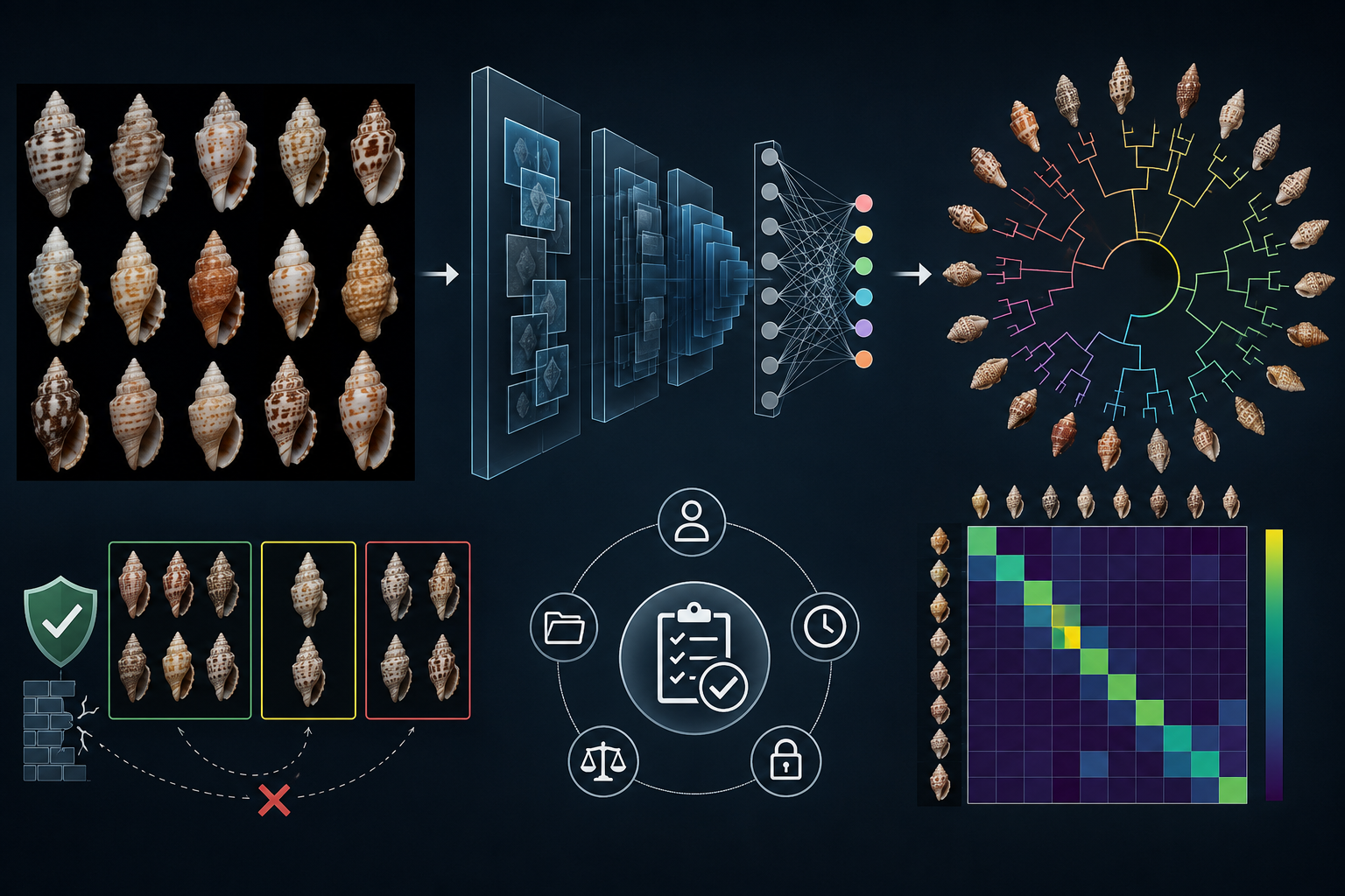
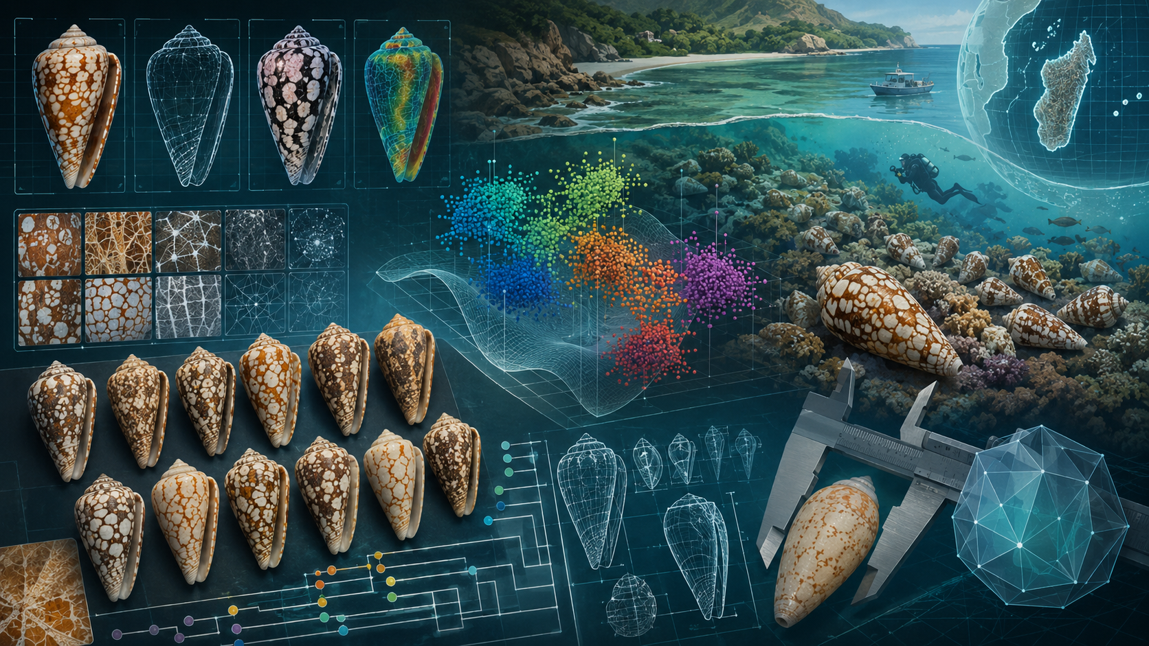
Here we apply this framework to a frozen photographic dataset of 1,000 physical specimens associated with the C. pennaceus complex. Shell phenotype is quantified using interpretable physical and image-derived traits together with frozen DINOv3 representations of the complete RGB phenotype, shell silhouette and luminance-normalized surface pattern. We first characterize phenotype structure and major observational effects, then use sufficiently represented currently accepted species as empirical benchmarks for morphological differentiation from an operational C. pennaceus sensu-stricto reference. Historical synonyms and unresolved forms are evaluated within the same framework. We further ask whether differentiation is integrated across shell shape and surface phenotype, whether individual specimens show discordant or mosaic combinations of these components, and whether internal variation within operational C. pennaceus sensu stricto supports recurrent discrete morphological components rather than continuous heterogeneity. The objective is not to delimit species from shell photographs alone, but to identify repeatable phenotype structure that can subsequently be tested using type material, geographically replicated sampling and independent molecular, anatomical and ecological evidence.
Materials and methods
Study design and analytical framework
The study was designed as a morphology-based assessment of phenotypic variation within the Conus pennaceus complex. Three types of information were kept conceptually separate: current nomenclatural status, phenotype labels attached to individual specimens, and morphological evidence generated from the photographs. Current name status was reconciled against MolluscaBase/WoRMS and was used to organize the sequence of comparisons, but was not treated as morphological ground truth [1]. Morphological differentiation was therefore interpreted as evidence concerning shell phenotype rather than, by itself, as demonstration of reproductive isolation or independently evolving species lineages [15, 16].
Taxonomic comparisons followed an accepted-species-first design. An operational C. pennaceus sensu-stricto group provided the common reference. Phenotype labels corresponding to currently accepted species were evaluated first to establish an empirical range of morphological differentiation among recognized taxa. Names currently treated as synonyms and unresolved project-level forms were then evaluated with exactly the same statistical framework. No aggregate test of “accepted species” versus “synonyms” was performed, and no universal amount of morphological separation was assumed to define species status.
Dataset construction and image standardization
Photographs were assembled for specimens identified as C. pennaceus or as species and named forms historically associated with the complex. Records originated from 32 provider categories encompassing biodiversity repositories, online catalogues, auction records, field guides and project collections. The material therefore represents an observational convenience sample rather than a spatially randomized population survey. Each database record represented a putative physical specimen, with duplicate groups used when several records were known to represent the same shell.
Original photographs with available local files entered a standardized processing pipeline. Shell instances were detected and segmented with the project YOLO segmentation model, and every valid non-empty mask generated a candidate shell crop. Multiple-shell images were not resolved by automatically selecting one detection. Automated confidence and geometry flags were retained as quality-control diagnostics, but final image acceptance or rejection was based on manual reviewer judgement. No separate adult/juvenile or shell-condition eligibility rule was applied.
Anatomical view was assigned manually. Only dorsal and apertural views judged certain or probable were retained for morphological analysis; oblique, lateral, apical, basal and uncertain projections were excluded. Eligible shell masks were standardized to an apex-up orientation using the principal long axis of the segmented shell and the position of the maximum supported perpendicular width to resolve axis direction. Images were rotated but never horizontally reflected, and orientation results were visually reviewed and corrected where necessary. Dorsal and apertural observations remained separate because projection changes apparent shell geometry [2, 3].
Each accepted orientation generated three aligned visual representations. The RGB stream retained the complete oriented colour image; the shape stream contained the corresponding binary shell silhouette; and the pattern stream was derived from the RGB image by within-shell luminance normalization in CIELAB space, reducing global brightness variation while retaining spatial pigmentation structure. Image and mask operations used OpenCV [6], and colour normalization used the CIE L*a*b* representation [11]. Shape and pattern derivatives were reviewed independently, and only complete accepted RGB–shape–pattern lineages were admitted to feature extraction.
The frozen analytical dataset contained 2,385 accepted representation triplets. Repeated photographs of the same physical specimen in the same anatomical view were pooled, producing 1,862 specimen–view units from 1,000 physical specimens: 934 apertural and 928 dorsal. Both views were available for 862 specimens, while 72 had only an apertural view and 66 only a dorsal view. The physical specimen, rather than the photograph, was treated as the independent biological unit whenever the statistical procedure permitted specimen-level blocking.
Phenotype labels and frozen analytical cohort
Label provenance was preserved in two fields. The original_variant field stored a phenotype name reconstructed from the source record, whereas assigned_variant stored a later project assignment when one had been made. The effective analytical label was the assigned variant when present and otherwise the original variant. Specimens for which neither field contained a named phenotype constituted the operational C. pennaceus sensu-stricto reference group.
Manual phenotype review and reassignment were performed by a single reviewer. Source labels were preserved rather than overwritten, and information from project analyses was available during some reviews. A focused review of several well-represented phenotypes could additionally display cross-validated morphological resemblance scores, but these scores were advisory and did not assign labels automatically. Consequently, reviewer-assigned labels were treated as curated phenotype hypotheses rather than as an independent ground-truth dataset against which the same image-derived morphology could be validated.
The reviewed state was frozen. The cohort fixed specimen membership, phenotype assignment, specimen–view structure and embedding arrays in immutable versioned artifacts. The operational sensu-stricto group contained 595 physical specimens. Its designation is therefore operational and residual: it does not imply that every specimen was directly compared with type material or independently validated using molecular evidence.
Quantification of shell phenotype
Shell morphology was quantified using 41 physical and image-derived fields describing conventional dimensions, shell and spire geometry, pattern organization, pigmentation and colour. Stored maximum shell length originated from specimen metadata. Shell width was propagated from recorded length and image-derived long- and short-axis geometry and was therefore treated as an image-derived width estimate rather than an independent calliper measurement. Shape measurements were calculated from the accepted silhouette and included proportional width, spire and shoulder geometry, outline compactness, asymmetry and body taper. Pattern measurements described regional pattern density, banding, fragmentation, reticulation and luminance entropy, while colour measurements included lightness, saturation, chroma and hue-related properties. These measurements extend established quantitative treatments of Conus shell geometry [2, 3].
Measurements from repeated accepted photographs of the same specimen and view were averaged; mean hue was combined by circular mean. Missing or invalid measurements were not imputed. Four tent-like-element measurements and three rule-based colour-coverage variables were retained as exploratory fields, and two legacy variables were retained for audit purposes rather than counted as independent biological evidence. Exact definitions and computational thresholds for all 41 fields are provided in the Supplementary Methods.
Overall measured-phenotype structure was summarized using a prespecified primary trait space. After removal of derived, duplicated, constant, legacy and explicitly exploratory variables, 29 biological fields were retained. Mean hue was represented by sine and cosine coordinates [12], yielding 30 numerical inputs. PCA was performed after feature standardization on the 837 physical specimens with complete data for these inputs. Phenotype modules were used to aid biological interpretation of the resulting axes but were not assumed to constitute statistically independent character sets.
DINOv3 embeddings and dimensionality reduction
The RGB, shape and pattern representations were embedded separately using the pretrained DINOv3 ViT-S/16 model dinov3_vit_small_lvd1689m [4]. The encoder was frozen throughout feature extraction and was not trained or fine-tuned on the phenotype labels used in this study. Inputs were resized to 336 × 336 × 3 pixels. RGB and pattern images used bilinear resizing; binary silhouettes used nearest-neighbour resizing before replication over three channels. No augmentation was applied during feature extraction.
The class token of the DINOv3 output was retained as a 384-dimensional image embedding. L2-normalized embeddings from repeated photographs of the same specimen and anatomical view were averaged and normalized again to produce the specimen–view representation. Phenotype labels, provider, anatomical view, geography and taxonomic status were not supplied to the encoder.
The 384 embedding dimensions were standardized separately within RGB, shape and pattern streams before PCA. A separate PCA basis was fitted to each representation, and the smallest number of components reaching at least 85% cumulative variance was retained for primary statistical inference. This yielded 56 RGB PCs, 19 shape PCs and 57 pattern PCs. Consequently, statistical analyses used the complete retained multivariate subspace rather than only the first two components. Two-dimensional PCA, UMAP and t-SNE projections were used for visualization only and did not provide evidence for clustering or taxonomic separation.
Association of measured traits with embedding structure
To establish the biological content of the image-derived feature spaces, each measured trait was associated separately with every retained PC in each representation. For a given trait–PC comparison, both variables were residualized against geographic region, repository provider and anatomical view on the same complete set of valid specimen–view observations. Pearson correlation between the residuals defined the partial correlation r, and r2 was reported as shared residual variance for that specific trait–PC pair. This quantity was kept distinct from the PCA explained-variance ratio of the corresponding component.
Mean hue was first expressed as the shortest angular deviation from its circular centre before the linear partial-correlation calculation [12]. Two-sided analytic probabilities were corrected by the Benjamini–Hochberg procedure across all retained PCs within each trait and representation [21]. These calculations treated specimen–view units as analysis rows and adjusted for anatomical view but did not explicitly model residual pairing of dorsal and apertural observations from the same specimen. Interpretation therefore emphasized effect magnitude and coherent biological associations rather than statistical significance alone.
Anatomical view, provider and geographic structure
Anatomical view, repository provider and geography were examined before taxonomic-group differences were interpreted. View dependence was assessed directly in morphometric structure and through specimen-level sensitivity analyses. Provider-associated variation was evaluated in the embedding spaces and retained as a nuisance term in subsequent focal-label models because differences among image sources can reflect both biological sampling and photographic acquisition.
Broad geographic structure in the embedding spaces was evaluated using an earlier frozen cohort of 1,359 specimen–view units representing 703 physical specimens. Geographic groups comprised the Western Indian Ocean, Mascarene Islands, Red Sea and Persian Gulf, and Central Indo-Pacific. PERMANOVA [17] evaluated regional effects in models containing repository source, log shell length and a shell-length-missingness indicator, while PERMDISP [18] assessed differences in within-region multivariate dispersion. Residual permutations for geographic and length terms were restricted within repository source. Paired dorsal and apertural rows were not clustered in this archived analysis, and its results were therefore interpreted as view-resolved rather than as a whole-specimen permutation test.
A separate current analysis examined measured phenotype within Madagascar and Mozambique using three locality-based regions: Madagascar, northern Mozambique, and central/southern Mozambique. For view-dependent traits, one observation was retained per physical specimen, preferentially apertural and otherwise dorsal. An initial trait-by-trait screen used one-way ANOVA for scalar variables and a sine/cosine representation with 999 label permutations for hue; false-discovery-rate correction was applied across the 41 traits. The principal complete-case multivariate analysis standardized the measured phenotype and fitted repository source before geographic region. The marginal regional contribution was tested with 999 Freedman–Lane residual permutations restricted within provider source [14]. Regional dispersion was evaluated separately by PERMDISP. The archived embedding and current three-region analyses use different analytical populations and phenotype spaces; their variance components were therefore not pooled.
Morphological comparison of named phenotypes with Conus pennaceus sensu stricto
Each named phenotype was compared independently with the operational sensu-stricto reference; specimens carrying other named labels were excluded from that focal comparison. The same statistical model was applied whether the focal name represented a currently accepted species, a synonym or a project-level form. Taxonomic status therefore affected the order and interpretation of comparisons, not their statistical construction.
For embedding analyses, RGB, shape and pattern were tested separately using all retained PCs through the stream-specific 85% variance cutoff. The full multivariate model contained geographic region, repository source, anatomical view and the focal phenotype label, while the reduced model omitted the label term. Morphological differentiation was summarized using standardized centroid separation, marginal R2 attributable to the focal label and a multivariate pseudo-F statistic.
The same comparison was performed separately for each measured trait using a linear model containing geographic region, repository source, anatomical view and focal phenotype label. The focal-label coefficient was standardized by residual variation to provide an adjusted effect size, and marginal R2 quantified the additional variance attributable to the label. Mean hue was analysed jointly through sine and cosine coordinates rather than as a linear degree variable [12].
Statistical support for both embedding and measured-trait comparisons used 999 restricted Freedman–Lane residual permutations [14]. All residual rows belonging to the same physical specimen were exchanged together within blocks defined by repository source, geographic region and anatomical-view signature. Permutation probabilities used the plus-one convention [22]. Embedding probabilities were corrected by Benjamini–Hochberg FDR separately across focal labels within each of the RGB, shape and pattern streams, whereas measured-trait probabilities were corrected as one global family across all estimable focal-label × trait comparisons [21].
A comparison was computationally eligible when the focal group contained at least five physical specimens and at least eight relevant specimen–view observations. A stricter requirement of 10 independent physical specimens was imposed before a species- or form-level morphological interpretation was made; smaller groups were classified as underpowered irrespective of individual test results. For adequately sampled groups, descriptive study-level categories summarized the strength of the shell phenotype: a strong distinction required at least two supported embedding streams, maximum standardized centroid separation ≥ 0.75 and at least five supported non-legacy traits; a moderate distinction required at least two supported embedding streams, maximum separation ≥ 0.40 and at least three supported traits. Remaining supported results were termed limited. These categories are study-specific screening rules and not general species-delimitation thresholds. Because RGB and normalized pattern originate from the same photographs and are strongly related, agreement between them was interpreted as one surface-phenotype result rather than as two independent biological datasets.
Phenotype-module correspondence and specimen-level discordance
A separate label-independent analysis examined correspondence among outline shape and surface phenotype. All retained PCs were first residualized against repository source and anatomical view, after which adjusted dorsal and apertural observations were averaged within physical specimens. Geographic region and phenotype labels were deliberately not included in this adjustment. Correspondence was evaluated for shape–pattern, shape–RGB and pattern–RGB pairs.
Global correspondence was quantified with the RV/linear centered-kernel- alignment coefficient, with statistical support obtained from 199 whole-specimen permutations. Procrustes correspondence, Spearman correlation between complete pairwise Euclidean-distance profiles, and overlap among each specimen's ten nearest neighbours provided complementary descriptive measures. The calculation was also repeated separately for dorsal and apertural views as a projection sensitivity analysis.
Frozen phenotype labels were overlaid only after cross-representation correspondence had been calculated. Group-level standardized centroid effects were used descriptively to identify broadly integrated, shape-led or surface-led phenotype differentiation. At the individual level, a mosaic-discordance score combined disagreement in ten-neighbour membership with disagreement in ranked specimen-to-specimen distance profiles across the three representation pairs. The highest 10% of scores provided an exploratory inspection set rather than a biological class. Nearest named-group resemblance was calculated from adjusted phenotype centroids for labels with at least five specimens, but these resemblance values were descriptive and were not probabilities, classifiers or automatic reassignment rules. Morphological discordance was not interpreted as evidence of hybridization, introgression, convergence or any other evolutionary mechanism.
Continuity versus mixture within Conus pennaceus sensu stricto
Internal phenotype structure was investigated only within the 595 specimens whose operational sensu-stricto assignment had already been frozen. Historical form names and taxonomic status were not used during unsupervised discovery. Four phenotype spaces were evaluated: outline shape, normalized surface pattern, RGB phenotype and a joint shape–pattern space. RGB was not added to the primary joint space because its information was largely redundant with the normalized pattern representation. For the joint analysis, centred shape and pattern blocks were separately scaled to equal Frobenius norm before concatenation, giving the two phenotype modules equal global numerical weight.
Each phenotype block underwent a second PCA restricted to the sensu-stricto specimens; components accounting for at least 90% of variance were retained, subject to a minimum of two and maximum of 15 dimensions. Diagonal-covariance Gaussian mixture models with K = 1–6 were then fitted. The Bayesian information criterion (BIC) [19] defined the candidate K, while five-fold held-out likelihood, component size, posterior assignment confidence, resampling stability and outlier sensitivity assessed robustness. Partition agreement was quantified using the adjusted Rand index [20].
Candidate structure was deliberately distinguished from a supported recurrent mixture. A multi-component candidate was promoted to supported K > 1 only when all prespecified criteria were satisfied: BIC selected more than one component; held-out likelihood improved over K = 1 by more than the combined standard error; the smallest component contained at least 5% of specimens; mean maximum posterior probability was at least 0.75; mean agreement across repeated 80% specimen subsamples was at least ARI = 0.70; removal of the most extreme 1% of specimens retained the same candidate component count; fewer than 50% of simulations selected multiple components under both Gaussian and Student-t5 continuous null models; and the larger of repository-source and view-availability normalized mutual information was below 0.25. Twenty simulations were evaluated for each continuous-null family. Failure of any required criterion resulted in supported K = 1, while the candidate solution remained available for descriptive interpretation.
Source holdout, locality holdout, separate-view recovery, locality composition and agreement between shape and pattern partitions were retained as additional robustness diagnostics but did not enter the locked supported-component rule. Associations between candidate components and measured traits or named-form resemblance were examined only after unsupervised component discovery and were therefore treated as post-hoc biological descriptions rather than as independent evidence used to create the partition.
Statistical inference and reporting
| Analysis | Principal unit | Adjustment / design | Primary inference |
|---|---|---|---|
| Trait–embedding correspondence | Specimen–view | Region + provider + anatomical view | Partial Pearson r; BH FDR across retained PCs within trait and stream |
| Archived embedding geography | Specimen–view | Region + shell length + length missingness + provider | PERMANOVA + PERMDISP |
| Madagascar–Mozambique geography | Physical specimen | Provider before three-region geography | 999 restricted Freedman–Lane permutations + PERMDISP |
| Focal phenotype vs sensu stricto | Physical-specimen residual cluster | Region + provider + anatomical view | Marginal R2, effect size, 999 restricted permutations, BH FDR |
| Cross-module correspondence | Physical specimen | Provider + anatomical view residualization | RV / linear CKA with 199 permutations; complementary descriptive correspondence metrics |
| Sensu-stricto mixture analysis | Physical specimen | Frozen sensu-stricto subset; source/view-adjusted phenotype blocks | BIC candidate K plus locked predictive, stability and continuous-null support criteria |
Unless otherwise specified, false-discovery-rate control used the Benjamini–Hochberg procedure [21], and permutation tests used plus-one probability estimates [22]. Effect sizes and variance components were reported alongside probabilities because statistical support alone was not treated as evidence of biological magnitude. Exact trait definitions, transformation parameters, quality-control warning thresholds, software and run identifiers, cohort manifests, dimensionality diagnostics, complete statistical tables and supplementary sensitivity analyses are documented in the Supplementary Methods.
Results
Measured traits and image embeddings described a multidimensional shell phenotype
The 1,000-specimen dataset contained substantial variation in shell size, outline geometry, surface pattern and colour. Thirty-eight of the 41 measured fields were available for all physical specimens; stored shell length and the derived physical-size variables were available for 837 specimens. Median shell length was 50.0 mm (interquartile range 46.0–54.8 mm), while median shell slenderness was 2.026 (1.885–2.154). Surface-pattern and colour measurements were generally more heterogeneous than several of the outline descriptors. For example, median dark-pattern coverage was 32.1%, with an interquartile range of 24.2–41.5%.
Several measured fields described the same or closely related biological information. Physical aspect ratio and shell slenderness were effectively identical (Spearman ρ > 0.999), and maximum-width position was identical to relative spire height (ρ = 1.000). Strong biological covariance was also evident among otherwise distinct traits: overall and middle-third pattern density were strongly correlated (ρ = 0.961), pattern density was negatively associated with mean lightness (ρ = −0.890), and relative spire height was negatively associated with spire angle (ρ = −0.855).
PCA of the 29-trait primary phenotype space confirmed that shell variation was distributed over several dimensions rather than dominated by a single morphological axis. PC1 accounted for 18.3% of standardized trait variance, PC2 for 16.9% and PC3 for 11.1%; together, the first three components represented 46.3% of total variance. The leading axes combined shell geometry, pigmentation and pattern organization. PC1 primarily contrasted dark, pattern-dense shells with lighter, more extensively white-patterned shells, whereas PC2 combined elongation and spire geometry with pattern density, reticulation and colour contrast.
The DINOv3 representations contained biologically interpretable information, but individual embedding PCs generally corresponded to combinations of measured traits rather than to single shell characters. RGB PC3 was strongly associated with physical aspect ratio (rpartial = −0.709; 50.3% shared residual variance), while shape PC2 was strongly associated with spire angle (rpartial = 0.685; 47.0%). Shape PC6 was associated with body taper (rpartial = 0.629; 39.5%), and shape PC1 with outline asymmetry (rpartial = 0.568; 32.2%). Surface phenotype was prominent on RGB PC1, including associations with saturation (rpartial = 0.610), regional pattern density and white coverage.
RGB and luminance-normalized pattern embeddings were especially similar. Across the 40 estimable measured traits, their trait-association profiles were nearly identical for the leading PCs, with coefficient correlations of 1.000, 0.994, 0.999, 0.996 and 0.997 for PCs 1–5, respectively. Thirty-one of 40 traits had the same strongest PC in the two representations. RGB and pattern were therefore treated as closely related representations of a common surface-phenotype module rather than as independent sources of biological evidence.
| Embedding axis | Measured trait | Partial r | Shared residual variance | PC variance | FDR q |
|---|---|---|---|---|---|
| RGB PC3 | Physical aspect ratio | −0.709 | 50.3% | 6.61% | <0.001 |
| RGB PC1 | Mean saturation | 0.610 | 37.2% | 15.15% | <0.001 |
| Shape PC2 | Spire included angle | 0.685 | 47.0% | 14.08% | <0.001 |
| Shape PC6 | Body taper ratio | 0.629 | 39.5% | 4.81% | <0.001 |
| Shape PC1 | Outline asymmetry | 0.568 | 32.2% | 20.42% | <0.001 |
Anatomical view and provider strongly structured the observed phenotype, whereas unique geographic effects were smaller
Non-taxonomic structure was evident before named phenotype groups were considered. The conspicuous two-band distribution previously observed for shell long-to-short-axis ratio versus cross-intersection position was strongly related to anatomical projection. Among the 600 orientation rows used in the original display, the smaller upper band contained 107 observations, of which 102 were dorsal and only five apertural. Association with band membership was stronger for provider (Cramér's V = 0.310) and anatomical view (V = 0.270) than for frozen phenotype label (V = 0.158) or geography (V = 0.127). The phenotype-label association was not supported in the row-level permutation analysis (p = 0.077).
Provider-associated structure was also substantial in the high-dimensional embeddings. In the archived geographic cohort, repository source accounted for 15.23% of RGB variance, 10.32% of shape variance and 14.91% of pattern variance in the region-plus-provider sensitivity models. After provider adjustment, broad geographic region accounted for 3.25%, 3.67% and 3.17%, respectively (all permutation p ≤ 0.001). Similar estimates were obtained when shell length and its missingness indicator were included in the full geographic model.
The current Madagascar–Mozambique trait analysis produced the same qualitative pattern within operational C. pennaceus sensu stricto. The complete-case analysis contained 268 physical specimens: 36 from Madagascar, 226 from northern Mozambique and six from central or southern Mozambique. Geography alone accounted for 11.41% of multivariate trait variance (p ≤ 0.001), but after repository source was entered first, the additional regional contribution fell to 1.86% (pseudo-F = 3.118, p = 0.037). Provider source accounted for 23.40%, leaving 74.74% as residual specimen-level variation. Regional dispersion was not supported at the 0.05 level in this sensu-stricto analysis (PERMDISP p = 0.056).
When all assigned phenotype groups were included, provider-adjusted regional variation was substantially larger (11.85%; p ≤ 0.001). Because this analysis included differences in the regional composition of named phenotypes as well as within-phenotype geographic variation, it was not interpreted as an estimate of geographic structure within C. pennaceus sensu stricto.
Accepted species spanned a broad range of morphological differentiation
Morphological recovery differed substantially among currently accepted species when each was compared with operational C. pennaceus sensu stricto. The strongest result was obtained for C. vezoi (N = 53). Standardized centroid separation was 1.363 in RGB (R2 = 9.41%, q = 0.002), 0.806 in shape (R2 = 4.26%, q = 0.003) and 1.354 in pattern (R2 = 9.33%, q = 0.002). Thirty-two measured fields were FDR-supported, with the largest effects involving reticulation-edge density, band count and pattern entropy. C. vezoi was therefore the clearest strongly differentiated multidimensional shell phenotype among the accepted species.
C. bazarutensis (N = 86) was also differentiated in all three representations, with its largest effect in shape (separation = 0.712; R2 = 6.61%, q = 0.003). Twenty-eight measured traits were supported, led by shoulder width, spire angle and shell slenderness. Its phenotype was therefore repeatable and strongly expressed in shell geometry but remained substantially overlapping with the sensu-stricto reference.
C. rubropennatus (N = 28) showed a different phenotype architecture. RGB and pattern separations were 0.454 and 0.451, respectively, compared with only 0.209 for shape. Twenty-five measured traits were supported, with the largest effects involving reticulation-edge density, saturation and brown coverage. The recovered differentiation was therefore predominantly associated with surface phenotype.
The remaining adequately sampled accepted species showed more limited differentiation. C. praelatus (N = 74) produced supported differences in all three embedding streams, but standardized separations remained small (0.181–0.251). C. quasimagnificus (N = 24) was supported only in shape (separation = 0.230, q = 0.044), with five supported traits. C. episcopus (N = 11) showed no supported multivariate embedding separation, although white-pattern coverage and saturation differed at trait level. C. ganensis (N = 6) and C. lohri (N = 2) were below the prespecified ten-specimen requirement and were therefore classified as underpowered rather than morphologically similar to C. pennaceus.
| Accepted species | N | RGB separation | Shape separation | Pattern separation | Supported traits | Assessment |
|---|---|---|---|---|---|---|
| C. vezoi | 53 | 1.363 | 0.806 | 1.354 | 32 | Strong multidimensional phenotype |
| C. bazarutensis | 86 | 0.479 | 0.712 | 0.478 | 28 | Moderate; shape-prominent and overlapping |
| C. rubropennatus | 28 | 0.454 | 0.209 | 0.451 | 25 | Moderate; predominantly surface phenotype |
| C. praelatus | 74 | 0.248 | 0.181 | 0.251 | 20 | Limited; supported but small effects |
| C. quasimagnificus | 24 | 0.139 | 0.230 | 0.140 | 5 | Limited; principally shape-supported |
| C. episcopus | 11 | 0.117 | 0.145 | 0.117 | 2 | Limited; trait-specific surface differences |
| C. ganensis | 6 | 0.331 | 0.241 | 0.315 | 0 | Underpowered |
| C. lohri | 2 | — | — | — | 0 | Underpowered |
The synonymized C. elisae phenotype was strongly differentiated
Among names not currently accepted as species within the C. pennaceus complex, only C. elisae was represented by enough independent specimens for an equivalent inferential assessment (N = 95). It showed FDR-supported differentiation in all three embedding representations and satisfied the study's strong morphological evidence criterion. Twenty-eight measured traits were supported after global correction.
The largest effects were concentrated in surface-pattern organization: overall pattern density (d = 2.69; R2 = 28.50%, q = 0.004), lower-third pattern density (d = 2.47; R2 = 21.90%), middle-third pattern density (d = 2.44; R2 = 25.61%), mean lightness (d = −2.14; R2 = 17.57%) and upper-third pattern density (d = 1.82; R2 = 15.95%); all five had q = 0.004. Shape was also significantly differentiated, so the phenotype was surface-dominated but not restricted to pigmentation and pattern.
The remaining synonymized and project-level labels were underpowered: marmoricolor contained eight specimens, C. rubiginosus seven, confusa five, C. colubrinus four and mimeticus two. Confusa showed support in two embedding streams despite its small sample, but no measured trait survived global FDR correction. These groups were retained as descriptive observations and were not assigned species- or form-level morphological conclusions. C. rubiginosus was considered separately because its current nomenclatural mapping is to C. episcopus.
Shell outline and surface phenotype formed partly independent morphological modules
Label-independent comparison of the three adjusted embedding representations revealed a pronounced difference between surface phenotype and outline shape. Pattern and RGB representations were almost equivalent at physical-specimen level: RV/linear CKA was 0.996, pairwise-distance Spearman ρ = 0.995 and mean ten-neighbour overlap was 85.7%. In contrast, correspondence between shape and pattern was much lower (CKA = 0.203, distance ρ = 0.340, neighbour overlap = 9.2%), as was correspondence between shape and RGB (CKA = 0.202, ρ = 0.339, neighbour overlap = 9.1%). All three CKA coefficients exceeded their whole-specimen permutation distributions (p = 0.005), indicating that shape–surface correspondence was weak but non-random.
The same two-module architecture was recovered when the anatomical views were analysed separately. RGB–pattern CKA remained 0.992 in apertural and 0.995 in dorsal observations, whereas the corresponding shape–surface coefficients were approximately 0.18 in both views. The relative independence of outline shape was therefore not an artefact of combining dorsal and apertural photographs.
Named groups differed in how their morphological signal was distributed across these modules. C. bazarutensis showed the clearest broadly integrated phenotype, with descriptive module effects of 0.80 for shape and 0.73 for both pattern and RGB. C. vezoi, by contrast, combined a substantial shape effect (0.76) with much larger pattern and RGB effects (both 1.45). C. rubropennatus was even more strongly surface-dominated (shape 0.31; pattern 0.78; RGB 0.79), and C. elisae showed the largest surface-biased profile (shape 0.52; pattern 1.46; RGB 1.45).
The modular structure was also visible at individual-specimen level. The highest 10% of mosaic-discordance scores defined an exploratory set of 100 specimens whose local neighbours and relative positions differed most strongly between phenotype representations. Within operational C. pennaceus sensu stricto, 60 of 595 specimens (10.1%) fell in this P90 set, close to the 10% expected from the cohort-wide definition. Individual specimens could therefore resemble one named phenotype in outline shape and another in surface pattern. Conversely, other specimens showed concordant shape, pattern and RGB resemblance. These individual discordances were retained as morphological observations rather than interpreted as evidence for a particular evolutionary mechanism.
Internal variation within Conus pennaceus sensu stricto was structured but did not support a recurrent discrete mixture
The unsupervised continuity analysis was restricted to the 595 physical specimens frozen as operational C. pennaceus sensu stricto before mixture discovery. In the primary equal-weight joint shape–pattern phenotype, BIC preferred a two-component Gaussian mixture over a one-component model. The candidate partition consisted of 539 specimens (90.6%) and 56 specimens (9.4%), with only 3.2% of specimens having maximum posterior assignment below 0.70.
The two-component candidate was reproducible. Relative to K = 1, held-out mean log likelihood improved by 0.335, mean ARI across repeated 80% specimen subsamples was 0.93, and leave-source and leave-locality-out analyses produced mean ARIs of 0.94 and 0.92, respectively. Removal of the most phenotypically extreme 1% of specimens retained candidate K = 2 and gave ARI = 0.84. Candidate membership showed little association with repository source (NMI = 0.06), locality (0.07) or anatomical-view availability (0.07).
Stability alone, however, did not establish that the two fitted components represented recurrent discrete morphotypes. The continuous-null analysis was decisive. BIC selected a single component in every Gaussian-null simulation, but selected more than one component in 100% of the Student-t5 heavy-tailed continuous simulations. The same behaviour occurred in the separate shape, pattern and RGB spaces. Thus, the tendency of the Gaussian mixture model to favour multiple components was compatible with approximation of a single heavy-tailed continuous distribution.
Additional results supported caution in interpreting the candidate split as a discrete phenotype boundary. Shape and normalized-pattern candidate assignments agreed poorly (ARI = 0.11), showing that the two phenotype modules did not divide the same specimens in the same way. Furthermore, no measured trait survived FDR correction in the post-hoc comparison of the two joint candidate components; the largest trait effect was only ε2 = 0.014. The joint candidate therefore lacked a strong conventional morphological diagnosis.
Because the prespecified heavy-tailed continuous-null requirement failed, the stable candidate K = 2 solution was not promoted to a supported mixture. The final result was therefore candidate K = 2, supported K = 1: internal phenotype variation was structured and heterogeneous, but the present shell data did not demonstrate recurrent discrete morphotypes within operational C. pennaceus sensu stricto.
Integrated morphological evidence differed from current nomenclatural rank
Taken together, the analyses recovered several distinct levels and architectures of shell differentiation among the sufficiently sampled phenotype labels. C. vezoi was the strongest accepted-species benchmark, while C. bazarutensis and C. rubropennatus showed moderate but overlapping differentiation expressed predominantly through shape and surface phenotype, respectively. C. praelatus, C. quasimagnificus and C. episcopus showed more limited photographic shell differentiation. In contrast, the currently synonymized C. elisae phenotype was strongly and multidimensionally differentiated and fell within the strongest part of the morphological range observed among accepted species.
Operational C. pennaceus sensu stricto was itself internally heterogeneous, but its variation did not satisfy the prespecified criteria for a recurrent discrete mixture. Thus, neither current species rank nor synonymy corresponded to a uniform level of photographic shell differentiation, and the observed phenotypes ranged from strongly multidimensional through module-specific and weakly differentiated to underpowered or internally heterogeneous outcomes.
Discussion
Multidimensional shell phenotype does not map uniformly onto current taxonomic rank
The principal result of this study is that morphological differentiation within the Conus pennaceus complex is both multidimensional and heterogeneous among named groups. Shell shape, surface pattern and colour covary, but they do not form a single axis of variation, and different phenotype groups are distinguished by different combinations of these components. This is consistent with earlier quantitative approaches to Conus morphology, in which shell proportions, spire geometry and landmark-based shape capture several partly independent dimensions of shell form rather than a single measure of morphological difference [2, 3].
The accepted-species-first analysis showed that current species rank does not correspond to a common degree of photographic shell differentiation. C. vezoi produced a strongly differentiated multidimensional phenotype, whereas C. bazarutensis and C. rubropennatus were repeatably but more moderately differentiated. Other accepted species showed considerably weaker shell separation, and two could not be assessed adequately because of small sample size. Accepted species therefore provided an empirical range of morphological outcomes rather than a numerical threshold that could be applied subsequently to decide whether another phenotype represents a species.
The result for C. elisae is particularly informative. Although the name is currently treated as a synonym of C. pennaceus [1], the adequately sampled elisae phenotype was strongly differentiated from the operational sensu-stricto reference. Its strongest differences concerned surface-pattern organization and lightness, but shape was also differentiated, placing elisae within the stronger part of the morphological range observed among currently accepted species. This result demonstrates that a historical name can remain associated with a recurrent and quantitatively recognizable shell phenotype after synonymization.
The converse is equally important: weak shell differentiation cannot be used to infer that two accepted taxa are conspecific. Species may overlap strongly in the external shell, may differ in characters not represented by the photographic protocol, or may be distinguished principally by molecular, anatomical or ecological evidence. Morphological diagnosability and species status are therefore related but non-equivalent properties [15, 16]. The present comparisons should consequently be interpreted as estimates of morphological differentiation among the sampled phenotypes, not as a morphology-derived reconstruction of current nomenclatural rank.
Phenotype modularity and mosaicism complicate simple morphological boundaries
The separation of the photographic phenotype into outline shape and surface representations revealed a clear modular structure. RGB and luminance-normalized pattern embeddings retained almost the same specimen-to-specimen relationships, whereas outline shape contributed substantially different information. The two surface representations should therefore be regarded as alternative analytical views of one broad pigmentation-pattern module rather than as independent evidence. In contrast, silhouette shape captures a more distinct component of phenotype.
Named groups differed in the relative contribution of these components. C. bazarutensis showed comparatively integrated shape and surface differentiation, while elisae, C. vezoi and especially C. rubropennatus were more strongly differentiated in surface phenotype than in outline shape. Thus, two phenotypes with a similar overall degree of visual diagnosability can differ substantially in the morphological architecture underlying that distinction. Describing the complex only by overall shell shape, or conversely only by conspicuous colour and pattern, would therefore discard biologically relevant information.
The same architecture was evident at individual-specimen level. Some shells occupied similar morphological neighbourhoods in shape and surface spaces, whereas others resembled different named groups in different phenotype modules. Such morphological mosaicism provides a useful description of the shell itself, but it does not identify the evolutionary process that produced that combination. In particular, discordance among shape and surface representations cannot by itself establish hybridization, introgression, convergence or common ancestry.
Internal variation within operational C. pennaceus sensu stricto reinforces the need to distinguish morphological structure from discrete groups. The joint shape–pattern analysis repeatedly recovered a stable two-component Gaussian-mixture approximation, and this partition was robust to resampling, source and locality holdouts and removal of extreme specimens. Nevertheless, the same model-selection procedure routinely divided simulated heavy-tailed continuous distributions into several Gaussian components. The prespecified continuous-null criterion therefore failed, giving candidate K = 2 but supported K = 1.
This result does not imply morphological homogeneity. Rather, the sensu-stricto phenotype is structured and heterogeneous without providing convincing evidence, under the present decision rule, for recurrent discrete morphotypes. The distinction is important because clustering algorithms can produce reproducible partitions of continuously distributed non-Gaussian data. A stable cluster solution should therefore not automatically be translated into biological morphotypes, still less into candidate species.
Geographic signal occurs within strong observational structure
Geography has historically been important in interpretations of the C. pennaceus complex, particularly in the western Indian Ocean [5]. The present analyses confirm that geographic differentiation is detectable, but they also show why its magnitude must be interpreted cautiously. Anatomical projection accounted for much of the conspicuous two-band structure in a simple morphometric display, and repository provider explained substantially more embedding variance than broad geographic region. Within the current Madagascar–Mozambique sensu-stricto analysis, the unique regional contribution became small after provider adjustment.
Provider should not be interpreted as a biological cause. It is a composite property of the observational dataset and can encode photographic conditions, specimen selection, geographic collecting history, preparation practices and differences among collections. Its large statistical contribution instead indicates that analyses based on heterogeneous online imagery can contain substantial source structure even after shell segmentation and image standardization. Likewise, anatomical view is primarily a consequence of projection geometry rather than a biological population effect. Explicitly accounting for these factors was therefore necessary before apparent taxonomic or geographic separation could be interpreted.
The geographic findings do not support the stronger conclusion that geography is unimportant. Rather, the present convenience sample provides limited evidence that geography is the dominant organizer of shell morphology within operational C. pennaceus sensu stricto once provider structure is taken into account. Regional differentiation was much larger when all named phenotypes were analysed together, but that result can also reflect geographic differences in the composition of those phenotypes. Distinguishing within-lineage geographic variation from regional changes in phenotype-group frequencies will require geographically balanced sampling of independently identified material.
The available molecular evidence is compatible with geography being biologically relevant but does not resolve this issue. Pereira et al. detected mitochondrial geographic structure in a small Mozambican sample [23], while broader molecular and phylogenomic studies provide an increasingly robust evolutionary framework for Conidae [24, 25, 26]. Neither evidence base presently provides the geographically dense sampling required to determine whether the shell gradients and phenotype groups analysed here correspond to population structure, lineage boundaries, environmentally associated variation or combinations of these processes.
Interpretable morphometrics and deep embeddings provide complementary evidence
A methodological contribution of the study is that the DINOv3 representations were biologically characterized rather than treated solely as opaque high-dimensional features. Several embedding PCs showed strong associations with recognizable shell properties, including elongation, spire geometry, body taper, outline asymmetry, saturation and pattern density. At the same time, the strongest PCs were generally associated with several traits, showing that they represented composite phenotype dimensions rather than digital replacements for individual conventional measurements.
Conventional morphometrics and deep image representations therefore answer partly different questions. Explicit measurements identify which recognizable shell properties differ and retain quantities such as absolute size that may be weakened by image normalization. Embeddings, by contrast, can represent spatial combinations of contour, pigmentation, reticulation and other image structure that are difficult to summarize using a small predefined character set. Their use is particularly appropriate in the C. pennaceus complex, where differentiation often involves combinations of geometry and surface pattern rather than a single diagnostic trait. Frozen self-supervised representations provide this broader visual description without fitting the encoder itself to the phenotype labels subsequently analysed [4].
The two approaches are consequently complementary rather than competing. Direct measurements provide biological interpretability but necessarily sample selected properties of the shell; embeddings provide broader visual coverage but require interpretation and control for acquisition-related structure. Relating the two provides a route from high-dimensional morphological separation back to recognizable shell characters while preserving information not readily summarized by those characters.
The present trait–PC analysis establishes biological correspondence but not the completeness of that correspondence. It tested individual traits against individual embedding axes and therefore does not determine how much of the complete RGB, shape or pattern representation can jointly be predicted from the full trait catalogue. Answering that question would require a separate multivariate predictive analysis evaluated on held-out physical specimens. The results therefore support neither replacing conventional morphometrics with DINOv3 nor interpreting the embeddings as merely a transformed version of the measured traits.
Morphological hypotheses require independent taxonomic validation
The principal inferential limitation of this study is that all primary evidence derives from photographed shells. Shape measurements, colour and pattern traits, RGB embeddings, normalized-pattern embeddings and silhouette embeddings provide different descriptions of morphology, but they are not independent organismal evidence. Strong agreement among these analyses demonstrates a coherent shell phenotype; it does not demonstrate reproductive isolation, genetic independence or species status. Conversely, weak shell differentiation cannot exclude cryptic or otherwise externally similar evolutionary lineages [15, 16].
A second limitation concerns phenotype-label provenance. The focal analyses were performed on a frozen reviewed cohort in which some labels originated from source records and others were subsequently assigned or revised during project review. The operational sensu-stricto group is additionally a residual category comprising specimens without another effective phenotype label, rather than a sample independently verified against type material. These assignments are therefore curated phenotype hypotheses rather than an external taxonomic reference.
This limitation is particularly relevant because information from project analyses was available during some manual reviews, and the focused review of the principal adequately sampled groups could display cross-validated morphological resemblance scores. The frozen DINOv3 encoder itself remained independent of project labels: it was neither trained nor fine-tuned on the phenotype assignments. However, independence of the representation does not imply complete independence of the subsequent group definitions. Recovery of coherent morphology in groups affected by morphology-assisted review should therefore be interpreted as quantitative characterization of the curated phenotype hypotheses rather than as an independent validation of those assignments.
The corresponding provenance fields and audit history preserve this distinction and allow future reassessment, but genuinely independent taxonomic validation requires additional evidence. Comparison with type material is needed to establish the connection between a recovered phenotype and the historical name to which it is assigned. Molecular sampling can test whether morphological groups correspond to genetic or phylogenetic structure, while anatomical and ecological evidence can provide independent organismal characters [15, 16]. Geographically replicated sampling is also essential because the present dataset was assembled from heterogeneous providers rather than from a balanced population-sampling design.
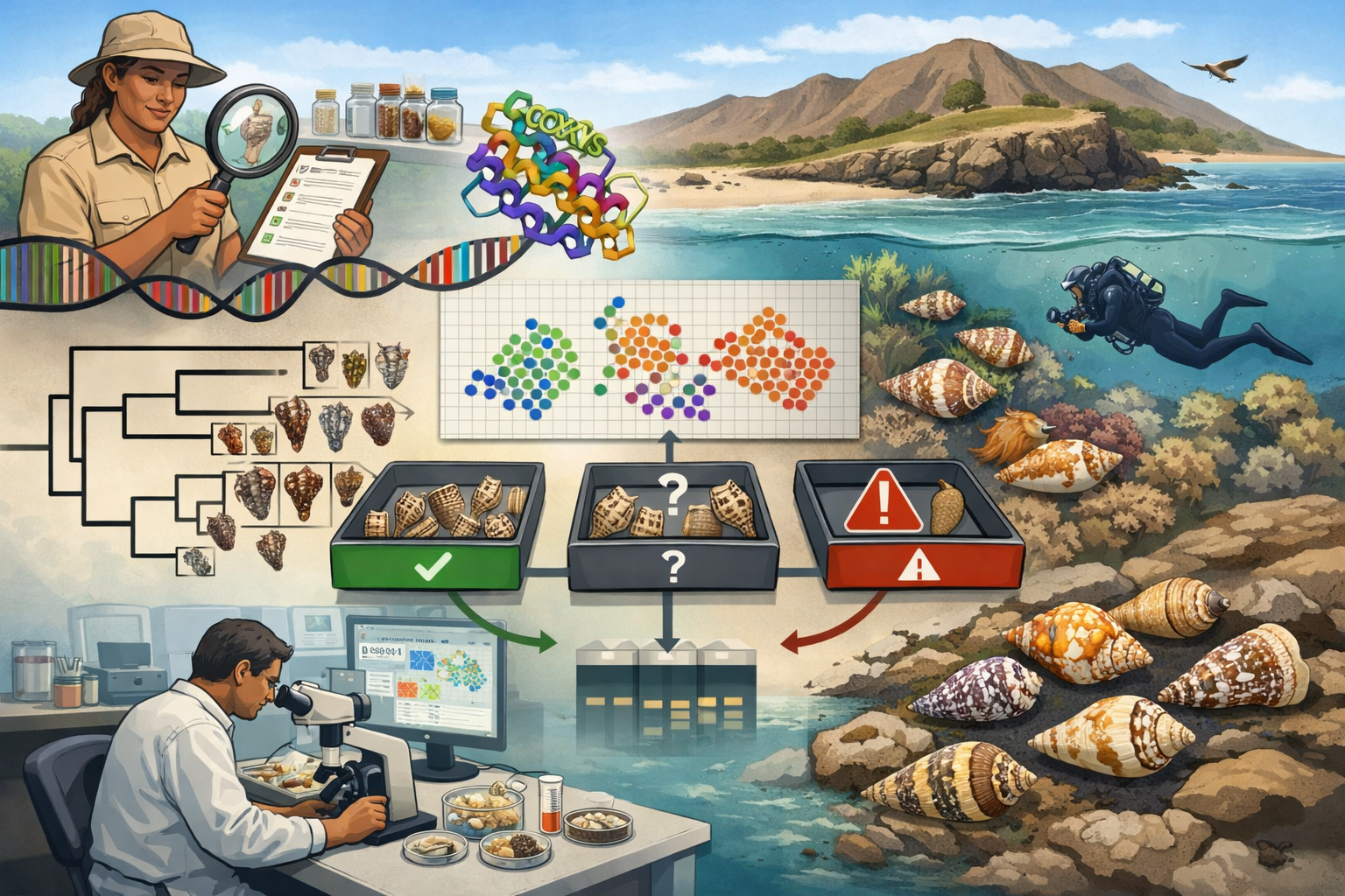
The strongest outcome of the present analysis is therefore not a revised species classification but a quantitative map of morphological hypotheses. It identifies phenotypes that are strongly or weakly differentiated, shows whether their distinction is concentrated in shell shape or surface phenotype, exposes individual mosaicism, and distinguishes stable internal heterogeneity from supported discrete mixture structure. In this role, interpretable morphometrics combined with self-supervised image embeddings can substantially refine the morphological component of integrative taxonomy, while type-based, molecular, anatomical, ecological and geographically replicated evidence remain necessary for decisions about evolutionary independence and nomenclatural status.
References
- [1] MolluscaBase eds. MolluscaBase/WoRMS. doi:10.14284/448 Accessed through the World Register of Marine Species on 14 August 2026
- [2] A J Kohn & A C Riggs. Morphometry of the Conus shell. Systematic Zoology, 24: 346–359 (1975)
- [3] R A L Cruz, M J R Pante & F J Rohlf. Geometric morphometric analysis of shell shape variation in Conus (Gastropoda: Conidae). Zoological Journal of the Linnean Society, 165: 296–310 (2012)
- [4] O Siméoni et al. DINOv3. arXiv:2508.10104 (2025)
- [5] W Korn, H-J Niederhöfer & M Blöcher. Conus pennaceus from Madagascar — a complex of geographical subspecies (Gastropoda: Conidae). Stuttgarter Beiträge zur Naturkunde, Serie A 610: 1–25 (2000)
- [6] K Pulli, A Baksheev, K Kornyakov & V Eruhimov. Real-time computer vision with OpenCV. Communications of the ACM, 55: 61–69 (2012)
- [7] S Suzuki & K Abe. Topological structural analysis of digitized binary images by border following. Computer Vision, Graphics, and Image Processing, 30: 32–46 (1985)
- [8] J Canny. A computational approach to edge detection. IEEE Transactions on Pattern Analysis and Machine Intelligence, PAMI-8: 679–698 (1986)
- [9] P Virtanen et al. SciPy 1.0: fundamental algorithms for scientific computing in Python. Nature Methods, 17: 261–272 (2020)
- [10] C E Shannon. A mathematical theory of communication. Bell System Technical Journal, 27: 379–423 (1948)
- [11] K McLaren. XIII—The development of the CIE 1976 (L* a* b*) uniform colour space and colour-difference formula. Journal of the Society of Dyers and Colourists, 92: 338–341 (1976)
- [12] P Berens. CircStat: a MATLAB toolbox for circular statistics. Journal of Statistical Software, 31: 1–21 (2009)
- [13] S H Hurlbert. Pseudoreplication and the design of ecological field experiments. Ecological Monographs, 54: 187–211 (1984)
- [14] A M Winkler, G R Ridgway, M A Webster, S M Smith & T E Nichols. Permutation inference for the general linear model. NeuroImage, 92: 381–397 (2014)
- [15] B Dayrat. Towards integrative taxonomy. Biological Journal of the Linnean Society, 85 (2005) .
- [16] K de Queiroz. Species Concepts and Species Delimitation. Systematic Biology, 56: 879–886 (2007) .
- [17] M J Anderson. A new method for non-parametric multivariate analysis of variance. Austral Ecology, 26: 32–46 (2001) .
- [18] M J Anderson. Distance-based tests for homogeneity of multivariate dispersions. Biometrics, 62: 245–253 (2006) .
- [19] G Schwarz. Estimating the Dimension of a Model. The Annals of Statistics, 6: 461–464 (1978) .
- [20] L Hubert & P Arabie. Comparing partitions. Journal of Classification, 2: 193–218 (1985) .
- [21] Y Benjamini & Y Hochberg. Controlling the False Discovery Rate: A Practical and Powerful Approach to Multiple Testing. Journal of the Royal Statistical Society: Series B (Methodological), 57: 289–300 (1995)
- [22] B Phipson & G K Smyth. Permutation P-values Should Never Be Zero: Calculating Exact P-values When Permutations Are Randomly Drawn. Statistical Applications in Genetics and Molecular Biology, 9: Article 39 (2010)
- [23] C M Pereira, J Rosado, S G Seabra, F Pina-Martins, O S Paulo & P J Fonseca. Conus pennaceus: a phylogenetic analysis of the Mozambican molluscan complex. African Journal of Marine Science, 32: 591–599 (2010)
- [24] N Puillandre, P Bouchet, T F Duda Jr, S Kauferstein, A J Kohn, B M Olivera, M Watkins & C Meyer. Molecular phylogeny and evolution of the cone snails (Gastropoda, Conoidea). Molecular Phylogenetics and Evolution, 78: 290–303 (2014)
- [25] N Puillandre, T F Duda Jr, C P Meyer, B M Olivera & P Bouchet. One, four or 100 genera? A new classification of the cone snails. Journal of Molluscan Studies, 81: 1–23 (2015)
- [26] S Abalde, M J Tenorio, J E Uribe & R Zardoya. Conidae phylogenomics and evolution. Zoologica Scripta, 48: 194–214 (2019)
- [27] J H Leal, G S Herbert, W Fenzan, A Avery & F Márquez. Geometric morphometrics reveal that Conus anabathrum Crosse, 1865 (Neogastropoda: Conidae) should be an accepted species. Journal of Molluscan Studies, 90: eyae019 (2024)